5.1
题目:我国1949-2008年每年铁路货运量数据如表5-9所示:
请选择适当的模型拟合该序列,并预测2009-2013年我国铁路货运量。
SAS程序
| data a; input volume@@; year=intnx(“year”,’01jan1949’d,_n_-1); format year year4.; cards; 54167 55196 56300 57482 58796 60266 61465 62828 64653 65994 67207 66207 65859 67295 69172 70499 72538 74542 76368 78534 80671 82992 85229 87177 89211 90859 92420 93717 94974 96259 97542 98705 100072 101654 103008 104357 105851 107507 109300 111026 112704 114333 115823 117171 118517 119850 121121 122389 123626 124761 125786 126743 127627 128453 129227 129988 130756 131448 132129 132802 ; proc arima data=a; identify var=volume; identify var=volume(1) stationarity=(adf); estimate p=1; forecast lead=5; run; |
答案:
该序列1阶差分后平稳,根据差分后序列的自相关图拖尾和偏自相关图1阶截尾特征,对该序列拟合ARIMA(1,1,0)模型,模型参数如下:
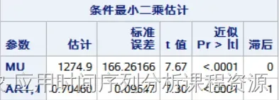
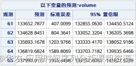
根据该模型,得到2009-2013年我国铁路货运量的预测值为:
5.2
1750-1849年瑞典人口出生率数据如表5-10所示。
请选择适当的模型拟合该序列的发展。
SAS程序
| data a; input year birth_rate; cards; 1750 9 1751 12 ┄(数据略) ; proc arima data=a; identify var=birth_rate stationarity=(adf); estimate p=1; run; |
答案
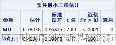
该序列adf检验平稳,根据自相关图和偏自相关图特征,可以识别为偏自相关图1阶截尾,拟合AR(1)模型。参数输出结果如下:
5.3
1867-1938年英国(英格兰及威尔士)的绵羊数量如表5-11所示(行数据)
- 确定该序列的平稳性
- 选择适当模型拟合该序列的发展
- 利用拟合模型预测1939-1945年英国绵羊的数量
SAS程序
| data a; input number@@; year=intnx(“year”,’01jan1867’d,_n_-1); format year year4.; cards; 2203 2360 2254 2165 2024 2078 2214 2292 2207 2119 2119 2137 2132 1955 1785 1747 1818 1909 1958 1892 1919 1853 1868 1991 2111 2119 1991 1859 1856 1924 1892 1916 1968 1928 1898 1850 1841 1824 1823 1843 1880 1968 2029 1996 1933 1805 1713 1726 1752 1795 1717 1648 1512 1338 1383 1344 1384 1484 1597 1686 1707 1640 1611 1632 1775 1850 1809 1653 1648 1665 1627 1791 ; proc arima data=a; identify var=number stationarity=(adf); identify var=number(1) stationarity=(adf); estimate p=3; estimate p=(1,3) noint; forecast lead=7; run; |
答案
- 根据时序图和adf检验结果可知,原序列非平稳,一阶差分后序列平稳。
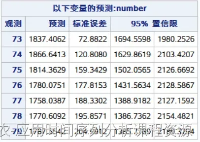
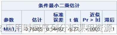
- 一阶差分后序列自相关图拖尾,偏自相关图3阶截尾,所以对原序列拟合模型ARIMA(3,1,0),参数输出结果显示2阶自相关系数与均值都不显著非零。所以最后拟合不带均值项的疏系数模型ARIMA((1,3),1,0),最后参数估计值输出结果如下
- 基于模型对1939—1945年英国绵羊的数量的预测为:
5.4
我国人口出生率、死亡率和自然增长率数据如表5-12所示。
- 分析我国人口出生率、死亡率和自然增长率序列的平稳性。
- 对非平稳序列选择适当的差分方式实现差分后平稳
- 选择适当的模型拟合我国人口出生率的变化,并预测未来10年的人口出生率
- 选择适当的模型拟合我国人口死亡率的变化,并预测未来10年的人口死亡率
- 选择适当的模型拟合我国人口自然增长率的变化,并预测未来10年的人口自然增长率。
SAS程序
| data a; input year birth_rate mortality ngr; cards; 1980 18.21 6.34 11.87 1981 20.91 6.36 14.55 1982 22.28 6.6 15.68 1983 20.19 6.9 13.29 1984 19.9 6.82 13.08 1985 21.04 6.78 14.26 1986 22.43 6.86 15.57 1987 23.33 6.72 16.61 1988 22.37 6.64 15.73 1989 21.58 6.54 15.04 1990 21.06 6.67 14.39 1991 19.68 6.7 12.98 1992 18.24 6.64 11.6 1993 18.09 6.64 11.45 1994 17.7 6.49 11.21 1995 17.12 6.57 10.55 1996 16.98 6.56 10.42 1997 16.57 6.51 10.06 1998 15.64 6.5 9.14 1999 14.64 6.46 8.18 2000 14.03 6.45 7.58 2001 13.38 6.43 6.95 2002 12.86 6.41 6.45 2003 12.41 6.4 6.01 2004 12.29 6.42 5.87 2005 12.4 6.51 5.89 2006 12.09 6.81 5.28 2007 12.1 6.93 5.17 2008 12.14 7.06 5.08 2009 11.95 7.08 4.87 2010 11.9 7.11 4.79 2011 11.93 7.14 4.79 2012 12.1 7.15 4.95 2013 12.08 7.16 4.92 2014 12.37 7.16 5.21 2015 12.07 7.11 4.96 2016 12.95 7.09 5.86 2017 12.45 7.11 5.32 ; proc arima data=a; identify var=birth_rate stationarity=(adf); identify var=birth_rate(1) stationarity=(adf); estimate p=0 q=0 noint; estimate q=1 noint; forecast lead=10; run; proc arima data=a; identify var=mortality stationarity=(adf); identify var=mortality(1) stationarity=(adf); estimate p=0 q=0 noint; forecast lead=10; run; proc arima data=a; identify var=ngr stationarity=(adf); identify var=ngr(1) stationarity=(adf); estimate p=0 q=0 noint; estimate p=1 noint; estimate q=1 noint; forecast lead=10; run; |
答案
- 我国人口出生率、死亡率和自然增长率序列均有显著线性趋势,为典型非平稳序列。
- 根据图检验和adf检验结果显示,我国人口出生率、死亡率和自然增长率序列的一阶差分后序列均平稳。
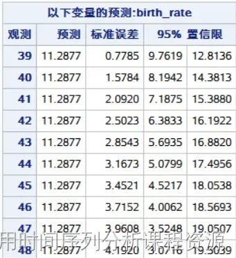
- 我国人口出生率可以拟合ARIMA(0,1,0)模型,也可以拟合ARIMA(0,1,1)模型。其中ARIMA(0,1,1)模型AIC,SBC更小一点。得到的拟合模型参数为
基于ARIMA(0,1,1)模型,预测1998年之后人口出生率未来十年的预测值为:
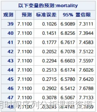
- 我国人口死亡率可以拟合随机游走模型ARIMA(0,1,0)。基于ARIMA(0,1,0)模型,预测1998年之后人口死亡率未来十年的预测值为:
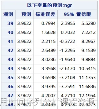
- (5)我国人口自然增长率可以拟合ARIMA(0,1,0)模型,ARIMA(1,1,0)模型,也可以拟合ARIMA(0,1,1)模型。其中ARIMA(0,1,1)模型AIC,SBC更小一点。得到的拟合模型参数为
基于ARIMA(0,1,1)模型,预测1998年之后人口自然增长率未来十年的预测值为:
5.5
某农场1867-1947年玉米和生猪的销售价、产量及农场工人平均收入如表5-13所示。
- 分析这几个序列的平稳性
- 对非平稳序列找到适当的差分阶数实现差分后平稳
- 选择适当的模型拟合这几个序列的发展,并做10年期序列预测
- 绘制拟合与预测效果图
SAS程序
| data a; input year maize_price maize_yield wages pig_price pig_yield; cards; 1867 6.85013 6.80239 6.57786 6.23245 6.28786 1868 6.73459 6.87109 6.57368 6.49678 6.25767 ┄(数据略) ; proc arima data=a; identify var=maize_price stationarity=(adf); identify var=maize_price(1) stationarity=(adf); estimate p=(11) noint; estimate q=(7) noint; forecast lead=10 id=year out=results1; run; proc gplot data=results1; plot maize_price*year=1 forecast*year=2 l95*year=3 u95*year=3/overlay; symbol1 c=black i=none v=star; symbol2 c=red i=join v=none; symbol3 c=green i=join v=none l=2; run; proc arima data=a; identify var=maize_yield stationarity=(adf); identify var=maize_yield(1) stationarity=(adf); estimate q=1; forecast lead=10 id=year out=results2; run; proc gplot data=results2; plot maize_yield*year=1 forecast*year=2 l95*year=3 u95*year=3/overlay; symbol1 c=black i=none v=star; symbol2 c=red i=join v=none; symbol3 c=green i=join v=none l=2; run; proc arima data=a; identify var=wages stationarity=(adf); identify var=wages(1) stationarity=(adf); estimate p=(1,13) noint; forecast lead=10 id=year out=results3; run; proc gplot data=results3; plot wages*year=1 forecast*year=2 l95*year=3 u95*year=3/overlay; symbol1 c=black i=none v=star; symbol2 c=red i=join v=none; symbol3 c=green i=join v=none l=2; run; proc arima data=a; identify var=pig_price stationarity=(adf); identify var=pig_price(1) stationarity=(adf) ; estimate p=3 noint; forecast lead=10 id=year out=results4; run; proc gplot data=results4; plot pig_price*year=1 forecast*year=2 l95*year=3 u95*year=3/overlay; symbol1 c=black i=none v=star; symbol2 c=red i=join v=none; symbol3 c=green i=join v=none l=2; run; proc arima data=a; identify var=pig_yield stationarity=(adf); identify var=pig_yield(1) stationarity=(adf); estimate p=(2,3,5) noint; forecast lead=10 id=year out=results5; run; proc gplot data=results5; plot pig_yield*year=1 forecast*year=2 l95*year=3 u95*year=3/overlay; symbol1 c=black i=none v=star; symbol2 c=red i=join v=none; symbol3 c=green i=join v=none l=2; run; |
答案
(1)玉米价格、玉米产量、工人薪水、生猪价格、生猪产量序列都不平稳,
(2)玉米价格、玉米产量、工人薪水、生猪价格、生猪产量序列一阶差分都实现平稳。
(3)-(4)分序列分析结果:
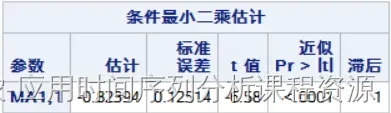
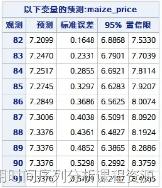
- 对玉米价格序列拟合疏系数模型ARIMA(0,1,(7)),参数估计值如下:

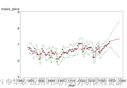
对玉米价格序列进行10期预测,预测值如下:
对玉米价格序列的拟合与预测效果图如下:
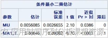
- 对玉米产量序列拟合模型ARIMA(0,1,1),参数估计值如下:
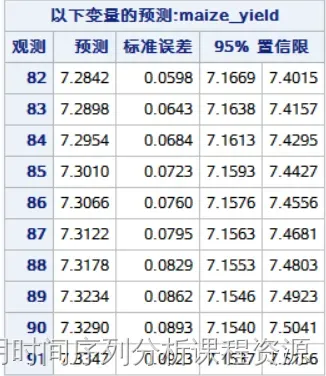
对玉米产量序列进行10期预测,预测值如下:
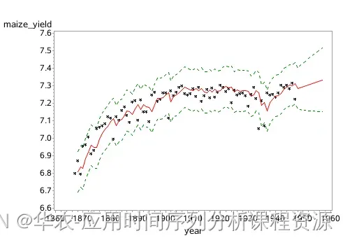
对玉米产量列的拟合与预测效果图如下:
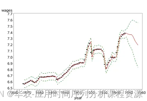
- 对工人薪水序列拟合疏系数模型ARIMA((1,13),1,0),参数估计值如下:
对工人薪水序列进行10期预测,预测值如下:
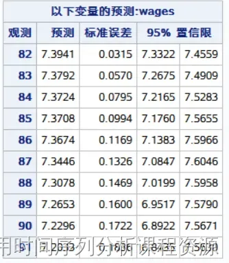
对工人薪水序列的拟合与预测效果图如下:
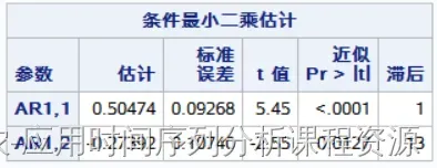
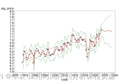
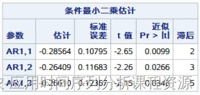
- 对生猪价格序列拟合模型ARIMA(3,1,0),参数估计值如下:
对生猪价格序列进行10期预测,预测值如下:
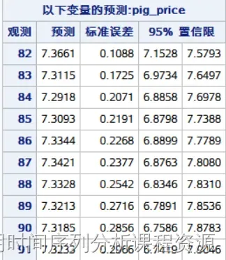
对生猪价格序列的拟合与预测效果图如下:
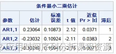
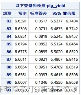
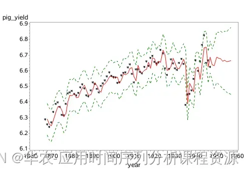
- 对生猪产量序列拟合疏系数模型ARIMA((2,3,5),1,0),参数估计值如下:
对生猪产量序列进行10期预测,预测值如下:
对生猪产量序列的拟合与预测效果图如下:
文章出处登录后可见!