mmdetection中的Mask Rcnn是一个很不错的检测网络,既可以实现目标检测,也可以实现语义分割。官方也有很详细的doc指导,但是对新手来说并不友好,刚好之前笔者写的mmlab系列里面关于可视化都还没有一个详细的文档,也在此一并介绍。
具体怎么制作自己的数据集和训练自己的模型教程如下:
mmdetect2d训练自己的数据集(一)—— labelme数据处理
mmdetect2d训练自己的数据集(二)—— 模型训练
通过上述两个教程,可以训练得到自己的config文件和checkpoints文件以及训练日志 xxx.log.json文件。接下来的可视化就是要用到这三个东西。
注:运行mmdetection的时候,我是用pycharm,这里有一个比较奇葩的bug,就是有时候我直接在terminal里面运行程序,会出现bug比如mmcv版本不对等,但是在RUN里面跑又可以了(别问怎么知道的,问就是卡了一周…)。所以出现bug的时候不要急着否定自己,多研究一下。
模型检测部署(检测结果可视化)
模型检测结果可视化有多种方式,这里介绍两种方法:1.调用api直接检测;2.用test.py进行检测。
1.使用test.py
运行test.py 必须要有config文件和checkpoint文件,其他为可选参数,具体如下:
python tools/test.py configs/myconfig.py checkpoints/last.pth \
--show --out result_file.pkl --show-dir result/test_result --eval segm

# --show 决定是否现实图片
# --out 将结果输出为pkl格式的文件
# --show-dir 将测试得到的文件存到目标文件夹下
# --eval 选择需要评估的指标,比如segm是分割的情况,这是mask rcnn网络会有这个结果,还有bbox等
2.调用API
在mmdet里面集成了很多现成的api也可以直接用来查看检测结果,这里写一个简单的调用方法。
from mmdet.apis import init_detector, inference_detector, show_result_pyplot
import cv2
import numpy as np

# config文件地址
config_file = 'others_ct/ct_head_mask_rcnn_r50_rpn_100_coco/mask_rcnn_r50_fpn_1x_coco.py'

# checkpoint文件地址
checkpoint_file = 'others_ct/ct_head_mask_rcnn_r50_rpn_100_coco/latest.pth'

# 选择使用的显卡
device = 'cuda:0'

# 模型载入
model = init_detector(config_file, checkpoint_file, device=device)

# 待检测的图片地址
img = 'data/coco_ct/val2017/Snipaste_2022-07-28_15-48-49.jpg'

# 检测结果输出
result = inference_detector(model, img)
#bbox_result, mask_result = result

# 现实检测结果
show_result_pyplot(model, img, result, score_thr=0.3)
3.对比自己的验证集标注
我之前都是用labelme直接看的,当然就显得b格不太够,mmdetection里面也可以直接看,用的browse_dataset.py,这个可以看训练集的,当然如果要看测试集的话,可以将config文件里面的data这个dict里面的train的dict中的ann_file和img_profix路径改成和val那个dict中的一样就好了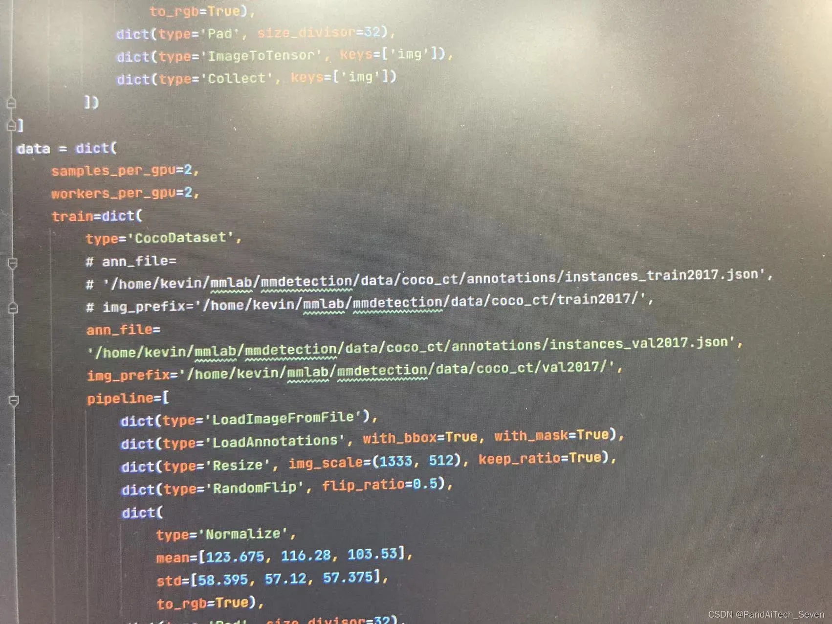
运行的时候,需要输入参数有config文件,以及--show # 如果你要现实每一张的话 ,--output-dir ../mydir # 浏览的图片可以保存到该地址下
这种现实办法有一个好处就是可以得到比较干净的对比图片,就是test.py得到预测的图片,这个得到标注的图片。但是如果想要将结果放在同一张图上进行展示,及标注和预测放在同一张图上的话,mmdetection也提供了对应的代码。使用tools/analyze_results.py即可。使用方法如下:
python tools/analysis_tools/analyze_results.py \
      ${CONFIG} \
      ${PREDICTION_PATH} \
      ${SHOW_DIR} \
      [--show] \
      [--wait-time ${WAIT_TIME}] \
      [--topk ${TOPK}] \
      [--show-score-thr ${SHOW_SCORE_THR}] \
      [--cfg-options ${CFG_OPTIONS}]

{CONFIG}: 是config文件路径
{PREDICTION_PATH}: 是test.py得到的pkl文件路径
{SHOW_DIR}: 是绘制的到的图片存放的目录
--show: 决定是否显示,不指定的话,默认为不显示
--wait-time时间的间隔,若为 0 表示持续显示
--topk: 根据最高或最低 topk 概率排序保存的图片数量,若不指定,默认设置为 20
--show-score-thr: 能够展示的概率阈值,默认为 0
--cfg-options: 如果指定,可根据指定键值对覆盖更新配置文件的对应选项
DICE(DSC)计算
我使用mask-rcnn这个网络的,想要计算语义分割结果理论上是可以直接用mmdetection里面的dice loss计算,但是我找了好几天没找到,主要是不知道怎么输出,所以就手动写了一个。主要原理是挨个计算标注的mask的面积、预测的mask的面积,以及二者的iou。
语义分割里 Dice = 2 * (A∩B) /(|A| + |B|)
但是这里有一点需要注意,我做的是单类别检测,且每张图最多会存在一个检测结果,如果有多类别的话,可能就需要对代码进行修改了,后续如果我用到的话也会更新的。
所以我是将mmdetection里面mask部分的numpy数组输出保存了。具体在image.py里面找到def imshow_det_bboxes函数,在判定segms的部分加上输出的指令:
if segms is not None:
	##############在原代码中的if语句里的开头部分添加该部分代码#################
	# 获取输出的的图片名称,这里一定要在test.py 和 browse_dataset.py的时候,选择保存文件,即必须有--show-dir和路径
	file_tmp = str(out_file)
	# 设置npy文件的名称
	file_name = file_tmp[:-3] + 'npy'
	# 将segms的numpy数组保存为npy文件
	np.save(file_name, segms)
	####################################################################
然后在运行上述的test.py文件和browse_dataset.py时,会在–show-dir下面,生成与图片同名的npy文件。计算dice就是要用到这部分文件。
因此具体代码如下:
import numpy as np
import os
# 存放预测结果的路径(前面test.py结果的--show-dir)
pred_root_path = '/home/kevin/mmlab/mmdetection/tools/result004'
# 存放标签的路径(前面dataset.py结果的--show-dir)
label_root_path = '/home/kevin/mmlab/mmdetection/tools/misc/ct_results'

# 读取预测结果路径下的文件
file_list_tmp = os.listdir(pred_root_path)
file_list = []
dice_list = []

for i in file_list_tmp:
	# 判定是否为npy文件
    if i[-3:] == 'npy':
    	# 获取预测的npy文件路径
        pred_path = pred_root_path + '/' + i
        # 获取同名的标签文件路径
        label_path = label_root_path + '/' + i
        print(pred_path)
        print(label_path)

        # 导入ndarray文件
        pred = np.load(pred_path)
        label = np.load(label_path)

        # 标签文件中的数组是Ture和False组成,需要变成1、0
        pred_1 = pred + 0
        # 因为browse得到的标签文件会有0.5的比例Flip来达到数据增强的目的,即图像会水平翻转
        # 所以产生的mask文件也有一半的概率是水平翻转过的,需要将其翻转回来
        pred_2 = pred_1[:,:,::-1]
        # 有时候检测为空但还是会有pred的npy文件,原因我也不清楚,所以这里是加了个判定,如果输出为空则直接跳过。
        # 预测的mask文件形状都是(n, 512, 512)形状的,n取决于预测的个数,我是单目标,所以最多只有一个。
        if pred_1.shape == (0, 512, 512):
            continue
        # 同上
        label = label + 0


        # 将 (1, 512, 512) 展平为 (262144,),目的是方便计算
        b1_1 = pred_1.flatten()
        b1_2 = pred_2.flatten()
        b2 = label.flatten()

        # 分别计算预测的和标签的两个mask部分的面积,因为翻转对面积不影响,这里只计算一次
        pred_area = np.sum(b1_1)
        label_area = np.sum(b2)

        # 计算IoU
        iou_pred_label_1 = b1_1 * b2
        iou_pred_label_2 = b1_2 * b2

        iou_area_1 = np.sum(iou_pred_label_1)
        iou_area_2 = np.sum(iou_pred_label_2)
        # print(iou_area_1, iou_area_2)

		# IoU小说明该图被翻转过了,因此选大的那个
        iou_area = max(iou_area_1, iou_area_2)
        print(iou_area)

		# 防止为空文件
        if (pred_area + label_area) > 0:
            dice = (2 * iou_area) / (pred_area + label_area)
        else:
            dice = 0
		# 将得到的dice加入list
        dice_list.append(dice)

# print("dice_list is:", dice_list)

# 求和前将list转为numpy数组
dice_np = np.array(dice_list)
dice_sum = np.sum(dice_np)

# 计算总共有多少张图片,因为一些检测为空,所以用的是browse的结果,由于结果包含图片和npy,所以除以2
pic_num = len(os.listdir(label_root_path)) / 2
print('num is:', pic_num)
# 计算平均Dice
Dice = dice_sum / pic_num
print('Dice is:', Dice)
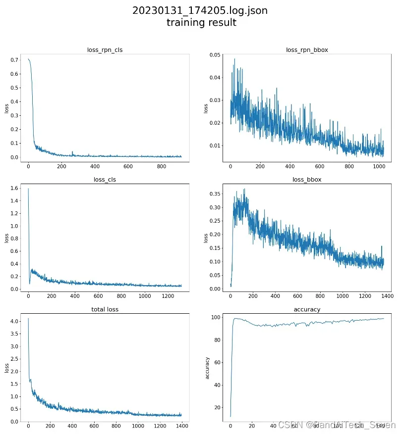
训练日志可视化
这一部分主要是将mmdetection训练得到的json文件可视化,代码主要源于github,具体哪一个忘记了(readme里面没有原址…)是专门做的mmdetection 结果可视化的,非常强!!。使用时如果出现keyerror的话,将json文件中第一行的env_info删掉就可以了。
import json
import matplotlib.pyplot as plt
import sys
import os
from collections import OrderedDict

class visualize_mmdetection():
    def __init__(self, path):
        self.log = open(path)
        self.dict_list = list()
        self.loss_rpn_bbox = list()
        self.loss_rpn_cls = list()
        self.loss_bbox = list()
        self.loss_cls = list()
        self.loss = list()
        self.acc = list()

    def load_data(self):
        for line in self.log:
            info = json.loads(line)
            # print('info:', info)
            if info['mode'] == 'train':
                self.dict_list.append(info)

        for i in range(1, len(self.dict_list)):
            for value, key in dict(self.dict_list[i]).items():
                # 读取每一行的信息
                loss_rpn_cls_value = dict(self.dict_list[i])['loss_rpn_cls']
                loss_rpn_bbox_value = dict(self.dict_list[i])['loss_rpn_bbox']
                loss_bbox_value = dict(self.dict_list[i])['loss_bbox']
                loss_cls_value = dict(self.dict_list[i])['loss_cls']
                loss_value = dict(self.dict_list[i])['loss']
                acc_value = dict(self.dict_list[i])['acc']
                # 将其保存至对应列表中
                self.loss_rpn_cls.append(loss_rpn_cls_value)
                self.loss_rpn_bbox.append(loss_rpn_bbox_value)
                self.loss_bbox.append(loss_bbox_value)
                self.loss_cls.append(loss_cls_value)
                self.loss.append(loss_value)
                self.acc.append(acc_value)
        # 清除list中的重复项
        self.loss_rpn_cls = list(OrderedDict.fromkeys(self.loss_rpn_cls))
        self.loss_rpn_bbox = list(OrderedDict.fromkeys(self.loss_rpn_bbox))
        self.loss_bbox = list(OrderedDict.fromkeys(self.loss_bbox))
        self.loss_cls = list(OrderedDict.fromkeys(self.loss_cls))
        self.loss = list(OrderedDict.fromkeys(self.loss))
        self.acc = list(OrderedDict.fromkeys(self.acc))

    def show_chart(self):
        plt.rcParams.update({'font.size': 15})

        plt.figure(figsize=(20, 20))

        plt.subplot(321, title='loss_rpn_cls', ylabel='loss')
        plt.plot(self.loss_rpn_cls)
        plt.subplot(322, title='loss_rpn_bbox', ylabel='loss')
        plt.plot(self.loss_rpn_bbox)

        plt.subplot(323, title='loss_cls', ylabel='loss')
        plt.plot(self.loss_cls)
        plt.subplot(324, title='loss_bbox', ylabel='loss')
        plt.plot(self.loss_bbox)
        plt.subplot(325, title='total loss', ylabel='loss')
        plt.plot(self.loss)
        plt.subplot(326, title='accuracy', ylabel='accuracy')
        plt.plot(self.acc)
        plt.suptitle((sys.argv[1][5:] + "\n training result"), fontsize=30)
        plt.savefig(('output/' + sys.argv[1][5:] + '_result.png'))


if __name__ == '__main__':
    x = visualize_mmdetection(sys.argv[1])
    x.load_data()
    x.show_chart()
使用时直接是:
python visualize.py xxxx.json
xxxx.json是生成的json文件,结果如下:
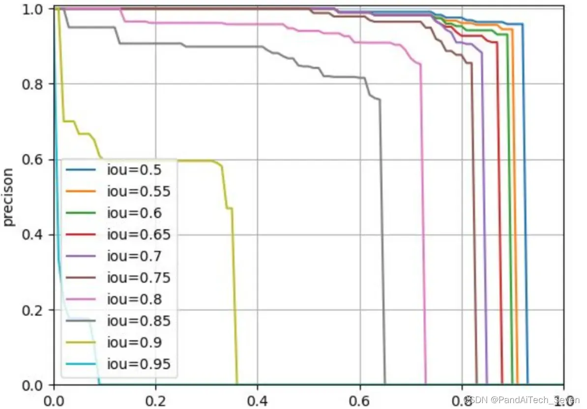
PR曲线绘制
不太确定mmdetection里面有没有内置的绘制PR曲线的代码,这是参考其他一些博主写的代码
import os
import mmcv
import numpy as np
import matplotlib.pyplot as plt

from pycocotools.coco import COCO
from pycocotools.cocoeval import COCOeval

from mmcv import Config
from mmdet.datasets import build_dataset

# config文件路径
CONFIG_FILE = '/home/kevin/mmlab/mmdetection/tools/others_ct/r18/mask_rcnn_r18_fpn_1x_coco.py'
# test.py得到的pkl文件路径
RESULT_FILE = '/home/kevin/mmlab/mmdetection/tools/r18_result.pkl'


## 对比不同网络之间的结果
#CONFIG_FILE_01 = '/home/kevin/mmlab/mmdetection/tools/others_ct/r18/mask_rcnn_r18_fpn_1x_coco.py'
#RESULT_FILE_01 = '/home/kevin/mmlab/mmdetection/tools/r18_result.pkl'

#CONFIG_FILE_02 = '/home/kevin/mmlab/mmdetection/others_ct/ct_head_mask_rcnn_r50_rpn_100_coco/mask_rcnn_r50_fpn_1x_coco.py'
#RESULT_FILE_02 = '/home/kevin/mmlab/mmdetection/tools/r50_result.pkl'

#CONFIG_FILE_03 = '/home/kevin/mmlab/mmdetection/tools/others_ct/ct_head_mask_rcnn_r101_rpn_100_coco/mask_rcnn_r101_fpn_1x_coco.py'
#RESULT_FILE_03 = '/home/kevin/mmlab/mmdetection/tools/r101_result.pkl'

# 绘制曲线
def plot_pr_curve(config_file, result_file, metric="bbox"):
    """plot precison-recall curve based on testing results of pkl file.

        Args:
            config_file (list[list | tuple]): config file path.
            result_file (str): pkl file of testing results path.
            metric (str): Metrics to be evaluated. Options are
                'bbox', 'segm'.
    """

    cfg = Config.fromfile(config_file)
    # turn on test mode of dataset
    if isinstance(cfg.data.test, dict):
        cfg.data.test.test_mode = True
    elif isinstance(cfg.data.test, list):
        for ds_cfg in cfg.data.test:
            ds_cfg.test_mode = True

    # build dataset
    dataset = build_dataset(cfg.data.test)
    # load result file in pkl format
    pkl_results = mmcv.load(result_file)
    # convert pkl file (list[list | tuple | ndarray]) to json
    json_results, _ = dataset.format_results(pkl_results)
    # initialize COCO instance
    coco = COCO(annotation_file=cfg.data.test.ann_file)
    coco_gt = coco
    coco_dt = coco_gt.loadRes(json_results[metric])
    # initialize COCOeval instance
    coco_eval = COCOeval(coco_gt, coco_dt, metric)
    coco_eval.evaluate()
    coco_eval.accumulate()
    coco_eval.summarize()
    # extract eval data
    precisions = coco_eval.eval["precision"]
    '''
    precisions[T, R, K, A, M]
    T: 是IOU的阈值,值为0-9,依次对应,[0.5 : 0.05 : 0.95],
    R: 召回率的阈值,[0 : 0.01 : 1], idx from 0 to 100
    K: 检测类别的索引,我只有1类,所以为0
    A: 检测的大小,对应 (all, small, medium, large), 索引值0-3
    M: 最大检测数量, 对应(1, 10, 100), 索引值0-2
    '''
    pr_array1 = precisions[0, :, 0, 0, 2]
    pr_array2 = precisions[1, :, 0, 0, 2]
    pr_array3 = precisions[2, :, 0, 0, 2]
    pr_array4 = precisions[3, :, 0, 0, 2]
    pr_array5 = precisions[4, :, 0, 0, 2]
    pr_array6 = precisions[5, :, 0, 0, 2]
    pr_array7 = precisions[6, :, 0, 0, 2]
    pr_array8 = precisions[7, :, 0, 0, 2]
    pr_array9 = precisions[8, :, 0, 0, 2]
    pr_array10 = precisions[9, :, 0, 0, 2]

	# 计算平均值 iou@0.5:0.95
    pr_array = pr_array1 + pr_array2 +pr_array3 +pr_array4 + pr_array5 + \
        pr_array6 + pr_array7 + pr_array8 + pr_array9 +pr_array10
    print(pr_array/10)

    x = np.arange(0.0, 1.01, 0.01)
    # 绘制PR曲线
    plt.plot(x, pr_array1, label="iou=0.5")
    plt.plot(x, pr_array2, label="iou=0.55")
    plt.plot(x, pr_array3, label="iou=0.6")
    plt.plot(x, pr_array4, label="iou=0.65")
    plt.plot(x, pr_array5, label="iou=0.7")
    plt.plot(x, pr_array6, label="iou=0.75")
    plt.plot(x, pr_array7, label="iou=0.8")
    plt.plot(x, pr_array8, label="iou=0.85")
    plt.plot(x, pr_array9, label="iou=0.9")
    plt.plot(x, pr_array10, label="iou=0.95")

    plt.xlabel("recall")
    plt.ylabel("precison")
    plt.xlim(0, 1.0)
    plt.ylim(0, 1.01)
    plt.grid(True)
    plt.legend(loc="lower left")
    # 保存图像
    plt.savefig('PR_r18.png')
    plt.show()

	# 只绘制ap @ 0.5:0.95
    # return pr_array/10


if __name__ == "__main__":
    plot_pr_curve(config_file=CONFIG_FILE, result_file=RESULT_FILE, metric="bbox")

    # pr_array_1 = plot_pr_curve(config_file=CONFIG_FILE_01, result_file=RESULT_FILE_01, metric="bbox")
    # pr_array_2 = plot_pr_curve(config_file=CONFIG_FILE_02, result_file=RESULT_FILE_02, metric="bbox")
    # pr_array_3 = plot_pr_curve(config_file=CONFIG_FILE_03, result_file=RESULT_FILE_03, metric="bbox")

    # x = np.arange(0.0, 1.01, 0.01)
    # plot PR curve
    # plt.plot(x, pr_array_1, label="r18")
    # plt.plot(x, pr_array_2, label="r50")
    # plt.plot(x, pr_array_3, label="r100")

    # plt.xlabel("recall")
    # plt.ylabel("precison")
    # plt.xlim(0, 1.0)
    # plt.ylim(0, 1.01)
    # plt.grid(True)
    # plt.legend(loc="lower left")
    # plt.savefig('PR_r18_r50_r101.png')
    # plt.show()
这边遇到了一个问题,就是使用plt保存图片时,必须要在ply.show前面,不然会保存为空白图像,因为它默认show完图像就被输出了,即没有可以保存的图像了。
得到结果图如下:
模型复杂度计算
这个官方文档就有python tools/analysis_tools/get_flops.py ${CONFIG_FILE} [--shape ${INPUT_SHAPE}]
得到结果如下:
==============================
Input shape: (3, 1280, 800)
Flops: 239.32 GFLOPs
Params: 37.74 M
==============================
对输出图像的处理
mmdetection检测或者预览的图像都是在image.py里面实现的,比如如果只是用mask rcnn来达到语义分割的效果,那么其实bbox和label输出就有点多余。同样是在def imshow_det_bboxes里面,把draw_bboxes和draw_labels注释掉就可以了
文章出处登录后可见!