一、二维图
1、柱形图
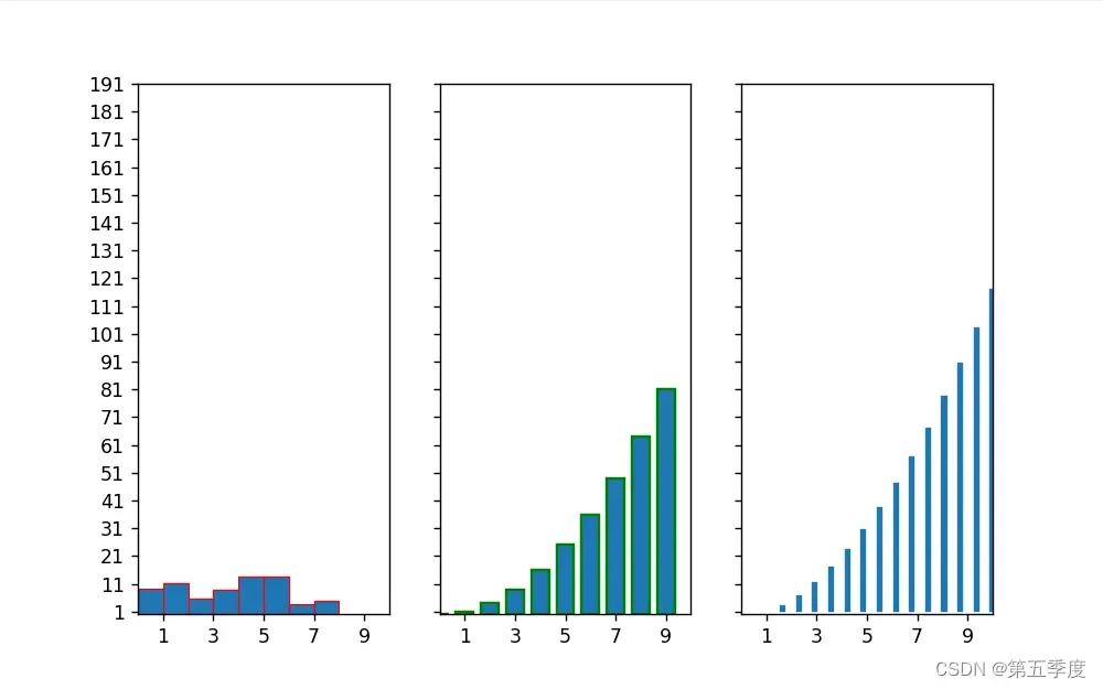
1.1、基础柱形图
import matplotlib.pyplot as plt
import numpy as np

# 模拟一些数据
np.random.seed(3)
x1 = 0.5 + np.arange(8)
y1 = np.random.uniform(2, 15, len(x1))
x2 = np.arange(10)
y2 = x2 ** 2
x3 = np.linspace(1,10,15)
y3 = x3 ** 2 + 2 * x3 - 2

# 获得图和坐标轴,图长宽比是8:5,图有1行3列,图中有3个坐标轴,这三个坐标轴共享y轴
fig, ax = plt.subplots(1, 3, figsize=(8,5), sharey=True)


# 为坐标轴设置边界和刻度
ax[0].set(xlim=(0, 10), ylim=(0, 100), xticks=np.arange(1, 11, 2), yticks=np.arange(1, 200, 10))
ax[1].set(xlim=(0, 10), ylim=(0, 100), xticks=np.arange(1, 11, 2), yticks=np.arange(1, 200, 10))
ax[2].set(xlim=(0, 10), ylim=(0, 100), xticks=np.arange(1, 11, 2), yticks=np.arange(1, 200, 10))

# 在坐标轴上画出三个柱形图
ax[0].bar(x1, y1, width=1, edgecolor="red", linewidth=0.7)
ax[1].bar(x2, y2, width=0.7, edgecolor="green", linewidth=1.4)
ax[2].bar(x3, y3, width=0.4, edgecolor="white", linewidth=2.1)

plt.show()
效果:
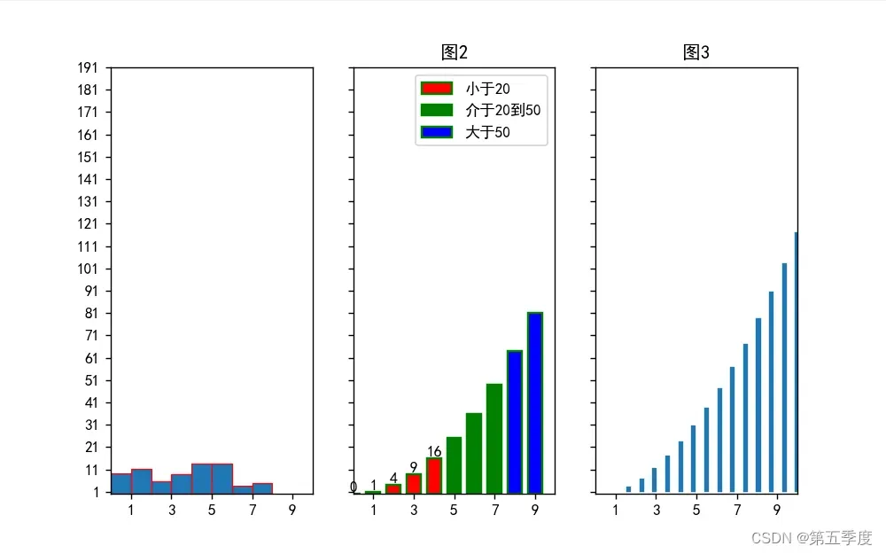
1.2、设置颜色、图例、图的标题
import matplotlib.pyplot as plt
import numpy as np

# 模拟一些数据
np.random.seed(3)
x1 = 0.5 + np.arange(8)
y1 = np.random.uniform(2, 15, len(x1))
x2 = np.arange(10)
y2 = x2 ** 2
x3 = np.linspace(1, 10, 15)
y3 = x3 ** 2 + 2 * x3 - 2

# 用来正常显示中文标签
plt.rcParams['font.sans-serif'] = ['SimHei']
# 用来正常显示负号
plt.rcParams['axes.unicode_minus'] = False
fig, ax = plt.subplots(1, 3, figsize=(8, 5), sharey=True)
ax[0].set(xlim=(0, 10), ylim=(0, 100), xticks=np.arange(1, 11, 2), yticks=np.arange(1, 200, 10))
ax[1].set(xlim=(0, 10), ylim=(0, 100), xticks=np.arange(1, 11, 2), yticks=np.arange(1, 200, 10))
ax[2].set(xlim=(0, 10), ylim=(0, 100), xticks=np.arange(1, 11, 2), yticks=np.arange(1, 200, 10))
ax[0].bar(x1, y1, width=1, edgecolor="red", linewidth=0.7)
ax[2].bar(x3, y3, width=0.4, edgecolor="white", linewidth=2.1)

# 为第二个柱形图添加颜色和标签。为每个x设置标签和颜色,有多少个x值,列表中就要有多少个元素。画完之后得到画的内容
container = ax[1].bar(x2[y2 < 20], y2[y2 < 20], width=0.7, edgecolor="green", linewidth=1.4, color="red",
                      label="小于20")
ax[1].bar(x2[np.logical_and(y2 >= 20, y2 < 50)], y2[np.logical_and(y2 >= 20, y2 < 50)], width=0.7, edgecolor="green",
          linewidth=1.4, color="green", label="介于20到50")
ax[1].bar(x2[y2 > 50], y2[y2 > 50], width=0.7, edgecolor="green", linewidth=1.4, color="blue", label="大于50")
# 在画的内容中显示y标签
ax[1].bar_label(container=container, label_type="edge")
# 有了标签之后,就可以显示图例
ax[1].legend(title="")
# 图2的标题
ax[1].set_title("图2")
# 图3的标题
ax[2].set_title("图3")

plt.show()
坐标轴对象可以设置要画的内容的标签,画完后可以返回一个绘制内容对象,绘制内容对象可以画出y标签的值。
效果如下:
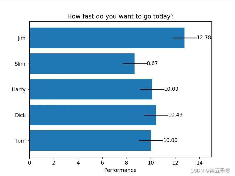
可以在坐标轴画图的时候指定误差棒。
import numpy as np
import matplotlib.pyplot as plt

# Fixing random state for reproducibility
np.random.seed(19680801)

# Example data
people = ('Tom', 'Dick', 'Harry', 'Slim', 'Jim')
y_pos = np.arange(len(people))
performance = 3 + 10 * np.random.rand(len(people))
error = np.ones(len(people))

fig, ax = plt.subplots()

# xerr是x轴方向的误差棒
hbars = ax.barh(y_pos, performance, xerr=error, align='center')
ax.set_yticks(y_pos, labels=people)
# ax.invert_yaxis()  # labels read top-to-bottom
ax.set_xlabel('Performance')
ax.set_title('How fast do you want to go today?')

# Label with specially formatted floats
ax.bar_label(hbars, fmt='%.2f')
ax.set_xlim(right=15)  # adjust xlim to fit labels

plt.show()
这里是将误差棒做成标签指示条了
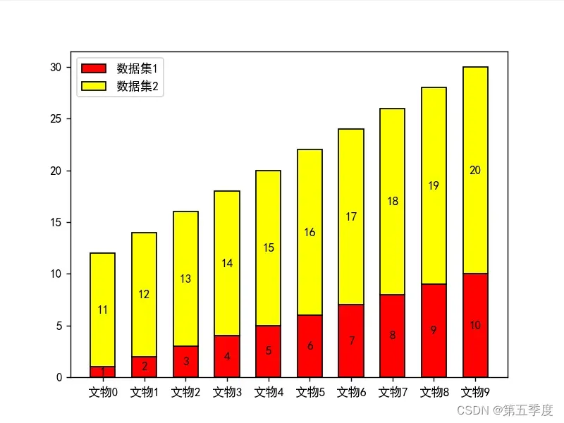
1.3、柱状堆积图
import matplotlib.pyplot as plt
import numpy as np

# 模拟一些数据
x = ['文物{}'.format(i) for i in range(10)]
y1 = np.arange(1,11)
y2 = np.arange(11,21)

# 用来正常显示中文标签
plt.rcParams['font.sans-serif'] = ['SimHei']
# 用来正常显示负号
plt.rcParams['axes.unicode_minus'] = False

fig, ax = plt.subplots(1,1)
container1=ax.bar(x,y1,color="red",label="数据集1",width=0.6,edgecolor="black")
# 关键在于画第二个内容时,要指定画的内容的底部是哪里。这里指定了第二个内容的底部是第一个内容的顶部
container2=ax.bar(x,y2,color="yellow",label="数据集2",bottom=y1,width=0.6,edgecolor="black")
ax.bar_label(container1,label_type="center")
ax.bar_label(container2,label_type="center")
ax.legend()

plt.show()
效果如下:
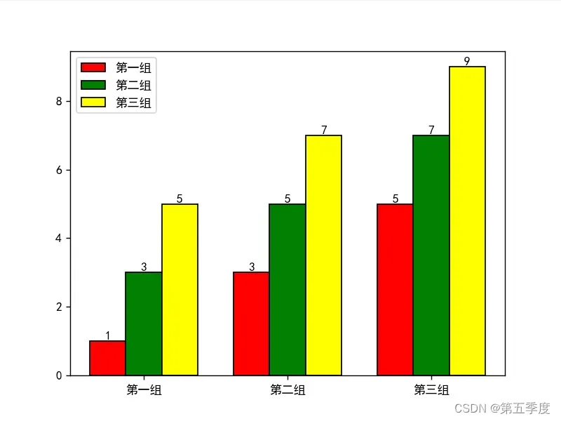
1.4、分组柱状图
最好首先确定每一组的x值、y值、在图中的位置、颜色、组别标签。后面比较好改。下面的代码只设定了x值、y值、颜色、组别标签,位置没有首先设置,是边循环边确定的。
import numpy as np
import matplotlib.pyplot as plt

gruop_label = ['第一组','第二组','第三组']
gruop_color = ['red','green','yellow']
x = np.arange(1,7,2)
y1 = np.arange(1,7,2)
y2 = np.arange(3,9,2)
y3 = np.arange(5,11,2)
y_list = [y1,y2,y3]

# 用来正常显示中文标签
plt.rcParams['font.sans-serif'] = ['SimHei']
# 用来正常显示负号
plt.rcParams['axes.unicode_minus'] = False
fig, ax = plt.subplots(1,1)
#画三次,每次都在x轴上偏斜一定距离画
width = 0.5
for index in range(len(y_list)):
    bar = ax.bar(x+index*width,y_list[index],edgecolor="black",label=gruop_label[index],width=width,color=gruop_color[index])
    ax.bar_label(bar,label_type="edge")
ax.legend()
plt.show()
效果如下:

会发现x轴的刻度错了。要把x轴的刻度设置成组别的标签,然后标签需要居中。
import numpy as np
import matplotlib.pyplot as plt

gruop_label = ['第一组','第二组','第三组']
gruop_color = ['red','green','yellow']
x = np.arange(1,7,2)
y1 = np.arange(1,7,2)
y2 = np.arange(3,9,2)
y3 = np.arange(5,11,2)
y_list = [y1,y2,y3]

# 用来正常显示中文标签
plt.rcParams['font.sans-serif'] = ['SimHei']
# 用来正常显示负号
plt.rcParams['axes.unicode_minus'] = False
fig, ax = plt.subplots(1,1)
#画三次,每次都在x轴上偏斜一定距离画
width = 0.5
for index in range(len(y_list)):
    bar = ax.bar(x+index*width,y_list[index],edgecolor="black",label=gruop_label[index],width=width,color=gruop_color[index])
    ax.bar_label(bar,label_type="edge")
ax.legend()
ax.set_xticks(x+1*width,gruop_label)
可以了。
二、三维图
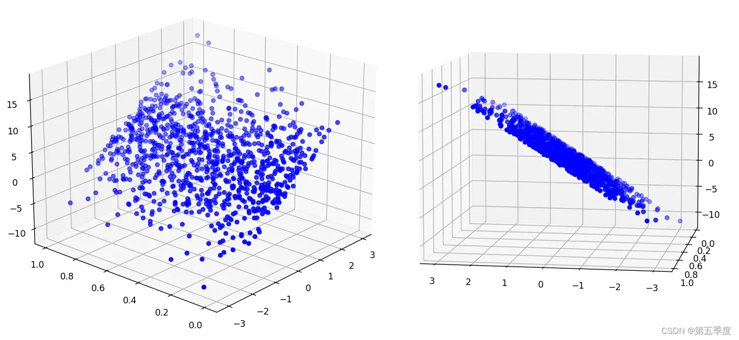
1、三维散点图
import numpy as np
import matplotlib.pyplot as plt

# 准备一些1000个点,这些点分布在一个平面上
x = np.random.normal(0,1,1000)
y = np.linspace(0,1,1000)
z = 4 * x + 5 * y + 1

fig = plt.figure()
ax = fig.add_subplot(111,projection='3d')
ax.scatter3D(x,y,z,color='blue')

plt.show()
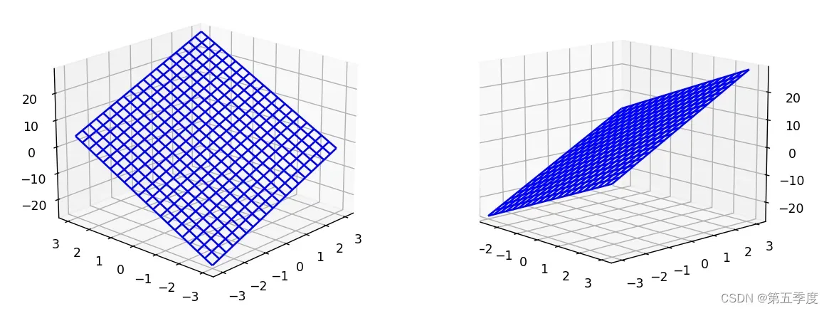
2、三维线框图
import numpy as np
import matplotlib.pyplot as plt

# 准备一些20个点,这些点分布在一个平面上(这些点要顺序生成,不能随机了)
x = np.linspace(-3,3,20)
y = np.linspace(-3,3,20)
# 把两个维度的数据形成网格
x, y =np.meshgrid(x,y)
# 利用网格得到z的数据(最好不要用到矩阵乘法……尽量使用标量*矩阵的形式吧)
z = 4 * x + 5 * y + 1

fig = plt.figure()
ax = fig.add_subplot(111,projection='3d')
ax.plot_wireframe(x,y,z,color='blue')

plt.show()
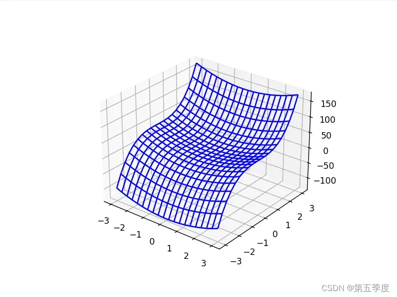
import numpy as np
import matplotlib.pyplot as plt

# 准备一些20个点,这些点分布在一个平面上(这些点要顺序生成,不能随机了)
x = np.linspace(-3,3,20)
y = np.linspace(-3,3,20)
# 把两个维度的数据形成网格
x, y =np.meshgrid(x,y)
# 利用网格得到z的数据(最好不要用到矩阵乘法……尽量使用标量*矩阵的形式吧)
z = 4 * (x ** 2) + 5 * (y ** 3) + 1

fig = plt.figure()
ax = fig.add_subplot(111,projection='3d')
ax.plot_wireframe(x,y,z,color='blue')

plt.show()
文章出处登录后可见!
已经登录?立即刷新