数字信号处理8：利用Python进行数字信号处理基础

我前两天买了本MATLAB信号处理，但是很无语，感觉自己对MATLAB的语法很陌生，看了半天也觉得自己写不出来，所以就对着MATLAB自己去写用Python进行的数字信号处理基础，我写了两天左右，基本上把matlab书上的代码全部用Python实现了，所以，今天贴的代码和图有些多，

要用到的包：

1、Scipy包：其中signal库，这个库是真的绝，很多信号处理的基础函数都有的，

2、numpy包：numpy包中也有很多进行信号处理的，比如说相关、卷积，都有相关函数

3、mmatplotlib包：这就不多说了，信号处理就是用它来展示的，这里主要用到的就是stem方法。

signal库我找了一下，csdn有个博主总结的很全，这是他的博客链接，可以看一看：

(1条消息) scipy.signal信号处理的库（笔记06）_scipy.signalku_月疯的博客-CSDN博客

然后，还可以看一下scipy官方的文档，里面也有很详细的介绍：

Signal processing (scipy.signal) — SciPy v1.10.1 Manual

这里我做了个目录，可以查看相应的方法：

目录

1、离散时间信号序列的表示：

 2、采样定理：

 3、简单离散信号序列：

 4、单位阶跃函数：

5、正弦信号序列：

6、实指数序列：

 7、复指数序列：

8、序列值累加和乘积：

9、序列反转、移位：

 10、信号的尺度变换：

 11、连续信号的奇偶分解：

12、奇函数和偶函数合并：

13、信号的微积分：

 14、积分：

15、卷积运算和相关计算

16、产生信号波形：

 17、连续矩形周期信号采样变成离散信号：

 18、随机函数，这个用numpy就可以直接生成：

 19、三角波，用signal的sawtooth：

 20、sinc曲线:

21、生成非周期三角波

 22、高斯脉冲的实现：

 23、脉冲序列发生器：

24、产生非周期方波：

25、连续时间信号的时域分析

（1）零状态响应：

 （2）冲激响应和阶跃响应：

 （3）各种信号的响应：

（4）连续时间信号的卷积：

26、离散时间系统：

27、离散时间系统的冲激和阶跃响应：

 28、卷积和运算，这都不用说啥了，前面都说过了：

 29、相关序列（自相关、互相关）：

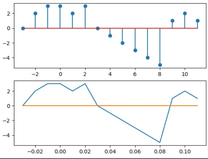
1、离散时间信号序列的表示：

import matplotlib.pyplot as plt
import numpy as np
from scipy import signal
N=np.linspace(-3,11,15,dtype=int)
x=np.array([0,2,3,3,2,3,0,-1,-2,-3,-4,-5,1,2,1])
dt=0.01
n=N*dt
fig=plt.figure()
ax1=fig.add_subplot(2,1,1)
ax1.stem(N,x)
ax2=fig.add_subplot(2,1,2)
ax2.plot(n,x)
ax2.plot(n,np.zeros(len(n)))

 2、采样定理：

#用10hz的采样频率采样
import matplotlib.pyplot as plt
import numpy as np
from scipy import signal
dt=0.01
n=np.linspace(0,89,90,dtype=int)
t=n*dt
f=10
x=np.sin(3*np.pi*f*t+0.5)#原始信号
dt=0.1
n=np.linspace(0,9,10,dtype=int)
t1=n*dt
x1=np.sin(3*f*np.pi*t1+0.5)# 采样后的信号
fig1=plt.figure()
ax1=fig1.add_subplot(3,1,1)
ax1.plot(t,x)
ax1.set_title('origional signal')
ax2=fig1.add_subplot(3,1,2)
ax2.plot(t,x)
ax2.plot(t1,x1,'*')
ax2.set_title('Sampling process')
ax3=fig1.add_subplot(3,1,3)
ax3.plot(t1,x1)
ax3.set_title('Sampling signal')
plt.show()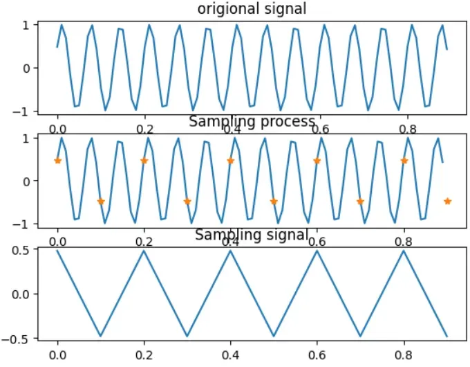

 3、简单离散信号序列：

import matplotlib.pyplot as plt
import numpy as np
from scipy import signal
n=50
x=np.zeros(n)
x[1]=1
xn=np.linspace(0,n-1,n,dtype=int)
fig1=plt.figure()
ax1=fig1.add_subplot(2,1,1)
ax1.stem(xn,x)
x[1]=0
x[10]=1
ax2=fig1.add_subplot(2,1,2)
ax2.stem(xn,x)
plt.show()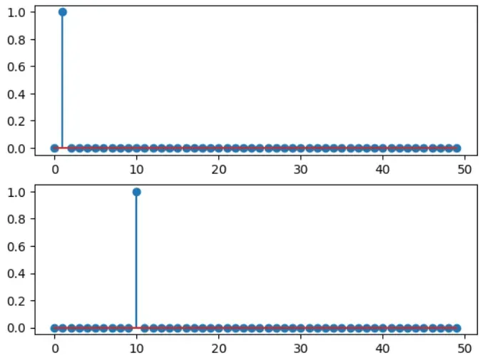

 4、单位阶跃函数：

这个我没有在signal里找到，但是我自己写了一个：

import matplotlib.pyplot as plt
import numpy as np
from scipy import signal
def u(n):
    if n>=0:
        r=1
    else:
        r=0
    return r
x=np.linspace(-10,10,21,dtype=int)
y=np.array([u(i)for i in x])
plt.stem(x,y)
plt.show()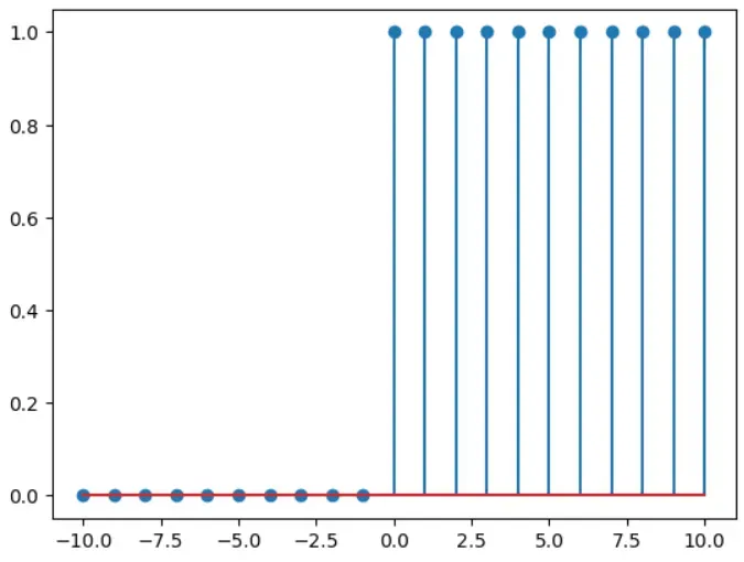

 很简单的，最简单的是递增序列，就是一个递增函数就行，比如说上面的x，他就是个递增序列：

plt.stem(x,x,'r')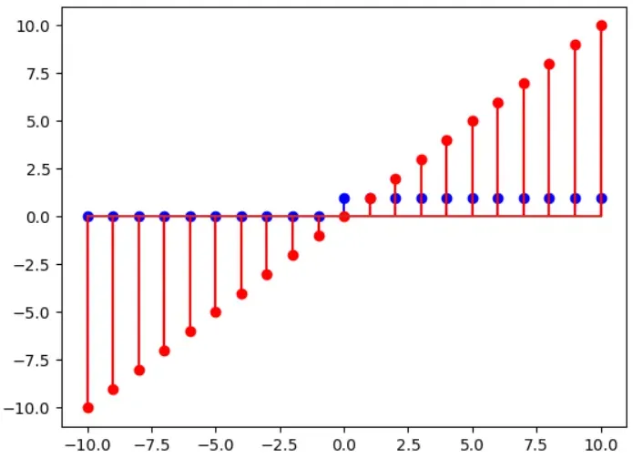

 蓝色的就是刚才的阶跃序列，

5、正弦信号序列：

这个也很简单，延续上面的代码：

# x=np.linspace(-10,10,21,dtype=int)
# z=np.linspace(-10,10,10000,dtype=float)
plt.stem(x,np.sin(x))
plt.plot(z,np.sin(z),'r')
plt.show()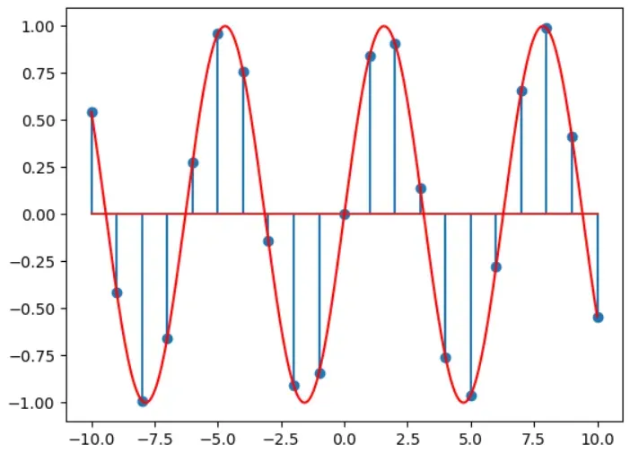

 可以看到，红色的连续信号和蓝色棉签棒的离散信号。

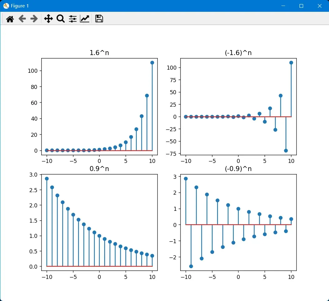
6、实指数序列：

numpy的power函数可以很简单的实现：

import matplotlib.pyplot as plt
import numpy as np
from scipy import signal
import sympy as sy
n=np.linspace(-10,10,21,dtype=int)
y1=np.power(1.6,n)
y2=np.power(-1.6,n)
y3=np.power(0.9,n)
y4=np.power(-0.9,n)
f=plt.figure()
ax1=f.add_subplot(2,2,1)
ax1.stem(n,y1)
ax2=f.add_subplot(2,2,2)
ax2.stem(n,y2)
ax3=f.add_subplot(2,2,3)
ax3.stem(n,y3)
ax4=f.add_subplot(2,2,4)
ax4.stem(n,y4)
ax1.set_title('1.6^n')
ax2.set_title('(-1.6)^n')
ax3.set_title('0.9^n')
ax4.set_title('(-0.9)^n')
plt.show()

 7、复指数序列：

import matplotlib.pyplot as plt
import numpy as np
from scipy import signal
import cmath
n=np.linspace(0,50,51,dtype=complex)
A=3
a=-1/9
b=np.pi/5
h=-1/9+np.pi/5j
x=A*np.exp(h*n)
f=plt.figure()
ax1=f.add_subplot(2,2,1)
ax1.stem(n,x.real)
ax2=f.add_subplot(2,2,2)
ax2.stem(n,x.imag)
ax3=f.add_subplot(2,2,3)
ax3.stem(n,abs(x))
ax4=f.add_subplot(2,2,4)
y=np.array([-cmath.phase(i) for i in x])#如果直接用phase的话，和matlab计算的angle是相反的，所以我这里为了和matlab一样，就用了-phase
ax4.stem(n,y)
ax1.set_title('real')
ax2.set_title('imag')
ax3.set_title('abs')
ax4.set_title('angle')
plt.show()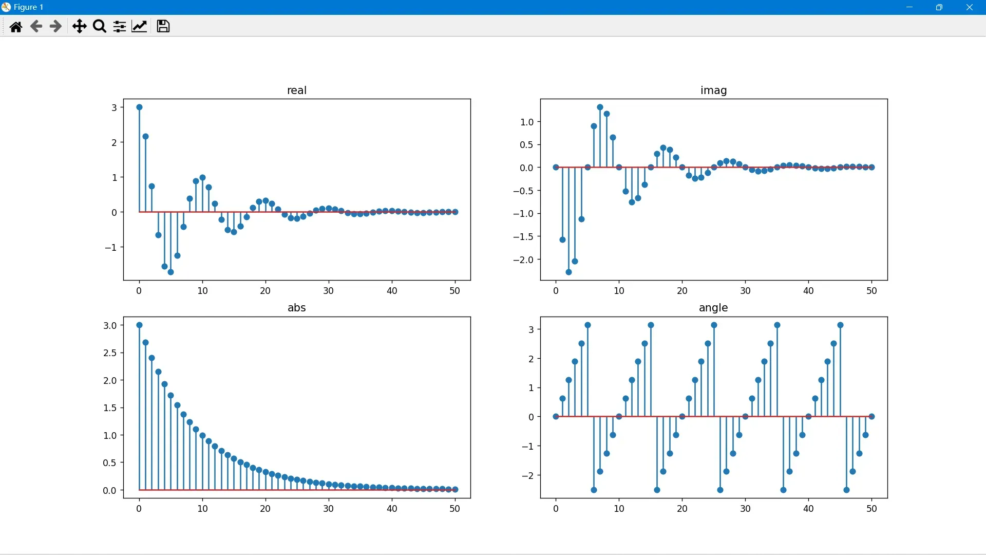

8、序列值累加和乘积：

这个就是常规的numpy操作，没啥意思

9、序列反转、移位：

反转的话，可以用[:：-1]或者也可以用y=np.flipud(x)，两者是一样的效果，信号移位就是，在一个信号序列前面或者后面加一个全零数组，前面加就是延迟，后面加就是提前：

# matlab中有一个函数较fliplr(x)来进行序列反转，但是，python会比这个更简单:两种方法：第一种是用列表反转的形式，第二种是用numpy的flipud函数执行
import numpy as np
import matplotlib.pyplot as plt
nx=np.linspace(-2,5,8,dtype=int)
x=np.linspace(2,9,8,dtype=int)
ny=-np.flipud(nx)
y=np.flipud(x)
print(ny)
print(y)
# ny=-nx[::-1]
# y=x[::-1]
fig=plt.figure()
ax1=fig.add_subplot(2,1,1)
ax1.stem(nx,x,'.')
ax1.axis([-6,6,-1,9])
ax1.grid(visible=True)
ax1.set_xlabel('n')
ax1.set_ylabel('x(n)')
ax1.set_title('origional sequence')
ax2=fig.add_subplot(2,1,2)
ax2.stem(ny,y,'.')
ax2.axis([-6,6,-1,9])
ax2.grid(visible=True)
ax2.set_xlabel('n')
ax2.set_ylabel('y(n)')
ax2.set_title('Inversion sequence')
plt.show()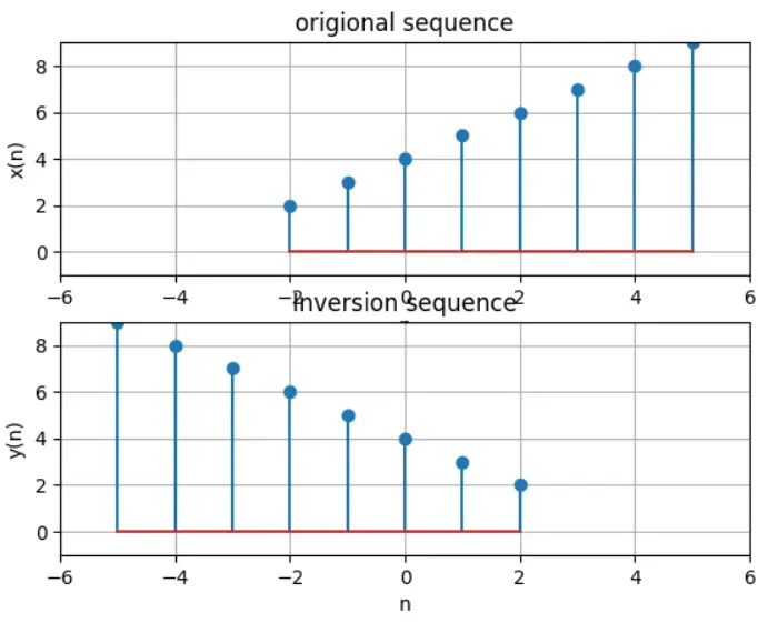

#序列位移：
import matplotlib.pyplot as plt
import numpy as np
nx=np.linspace(-2,5,8,dtype=int)
x=np.array([9,8,7,6,5,5,5,5])
y=x
ny1=nx+3
ny2=nx-2
fig=plt.figure()
ax1=fig.add_subplot(2,1,1)
ax1.stem(nx,x,'.')
ax1.axis([-5,9,-1,10])
ax1.grid(visible=True)
ax1.set_xlabel('n')
ax1.set_ylabel('x(n)')
ax1.set_title('origional sequence')
ax2=fig.add_subplot(2,2,3)
ax2.stem(ny1,y,'.')
ax2.axis([-5,9,-1,10])
ax2.grid(visible=True)
ax2.set_xlabel('n')
ax2.set_ylabel('y1(n)')
ax2.set_title('y1=(n+3)')
ax3=fig.add_subplot(2,2,4)
ax3.stem(ny2,y,'.')
ax3.axis([-5,9,-1,10])
ax3.grid(visible=True)
ax3.set_xlabel('n')
ax3.set_ylabel('y2(n)')
ax3.set_title('y2=(n-2)')
plt.show()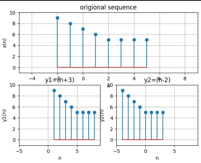

 10、信号的尺度变换：

把信号的横坐标压缩或者扩展：

t = np.linspace(-4, 4, 8000, dtype=float)
T = 2
f = np.zeros((8000),dtype=float)
t1=2*t
f1=np.zeros((8000),dtype=float)
for i in range(len(t)):
    if ((-1 <= t[i]) & (t[i] <= 1)).any():
        f[i] = 1
for i in range(len(t1)):
    if ((-0.5 <= t1[i]) & (t1[i] <= 0.5)).any():
        f1[i] = 1
fig=plt.figure()
ax1=fig.add_subplot(2,1,1)
ax1.plot(t,f)
ax1.axis([-4,4,-0.5,1.5])
ax2=fig.add_subplot(2,1,2)
ax2.plot(t1,f1)
ax2.axis([-4,4,-0.5,1.5])
plt.show()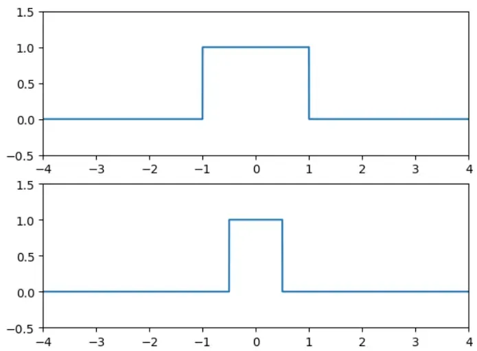

 11、连续信号的奇偶分解：

我们都知道，一个信号可以分解成一个偶分量和一个奇分量：

#连续信号的奇偶分解：
#对于一个信号f(n)来说，奇信号：1/2[f(t)-f(-t)]偶信号：1/2[f(t)+f(-t)]
t=np.linspace(-8,8,100000)
f=np.cos(t+1)+t
f1=np.cos(-t+1)-t
g=1/2*(f+f1)
h=1/2*(f-f1)
fig=plt.figure()
ax1=fig.add_subplot(3,1,1)
ax1.plot(t,f)
ax1.set_title('origional signal')
ax2=fig.add_subplot(3,1,2)
ax2.plot(t,g)
ax2.set_title('odd signal')
ax3=fig.add_subplot(3,1,3)
ax3.plot(t,h)
ax3.set_title('even signal')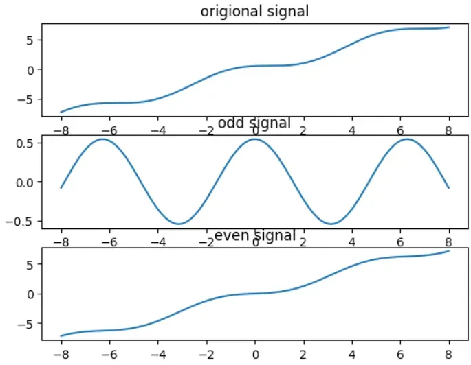

12、奇函数和偶函数合并：

还是上面的

#将上面的两个奇偶分量合并成原函数：就是反向操作一波，也可以用g-h
t=np.linspace(-8,8,100000)
f=np.cos(t+1)+t
f1=np.cos(-t+1)-t
g=1/2*(f+f1)
h=1/2*(f-f1)
z=g+h
l=h-g
fig=plt.figure()
ax1=fig.add_subplot(4,1,3)
ax1.plot(t,z)
ax1.set_title('origional signal')
ax1=fig.add_subplot(4,1,4)
ax1.plot(t,l)
ax1.set_title('origional signal')
ax2=fig.add_subplot(4,1,1)
ax2.plot(t,g)
ax2.set_title('odd signal')
ax3=fig.add_subplot(4,1,2)
ax3.plot(t,h)
ax3.set_title('even signal')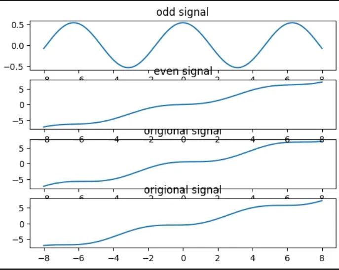

 多画了一个原函数，将就着看吧

13、信号的微积分：

这个里面有一个heaviside函数，matlab有，但是python没有，然后我就把它自己实现了，要用的可以直接用：

import matplotlib.pyplot as plt
import numpy as np
import sympy as sp
from scipy import signal
import sympy.plotting as syp
def heaviside(x):
    if x==0:
          r=0.5
    elif x>0:
          r=1
    elif x<0:
          r=0
    return r
#本来要用的，但我们没有用heaviside函数
t=sp.symbols('t')
f=sp.Function('f')(t)
f=t*t+2*t-1
f1=f.diff(t)#一阶导
f2=f.diff(t,t)#二阶导
f3=f.diff(t,t,t)#三阶导
syp.plot(f,f1,f2,f3,(t,-1,2))

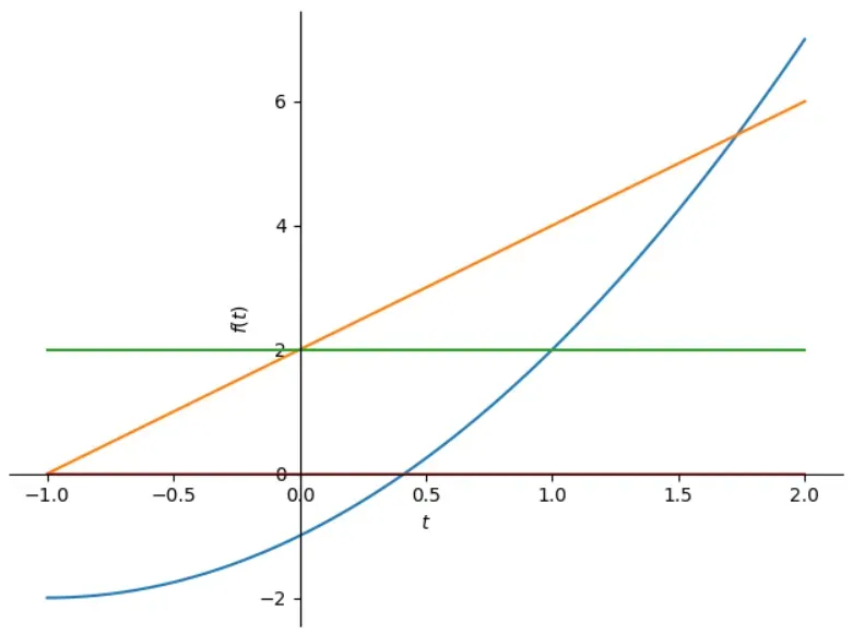
 14、积分：

这里用的是：

import sympy as sy
t,f=sy.symbols('t,f')
f=2*t+2
intt=sy.integrate(f,t)
print(intt)
syp.plot(intt,(t,-7,5))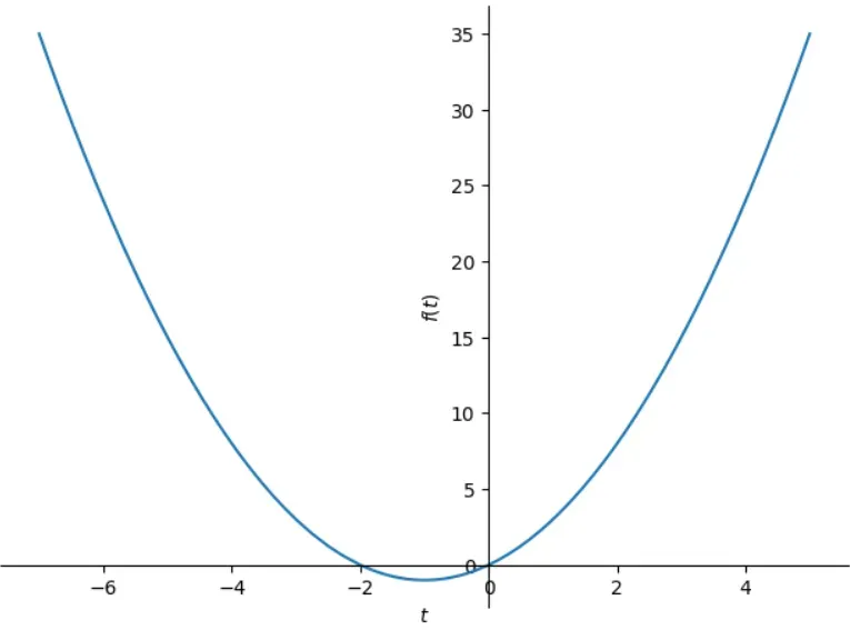

 当然，微积分这里比较水，以为找个很好看的函数很麻烦

15、卷积运算和相关计算

连续信号和离散信号都一样，我们可以用numpy中的convolve函数，singal中也有这个函数，直接计算就可以，这里给例子：

#离散时间信号的卷积和运算
import matplotlib.pyplot as plt
import numpy as np
from scipy import signal
def uDt(n):
    if n>=0:
        y=1
    else:
        y=0
    return y
nx=np.linspace(-1,5,7,dtype=int,endpoint=True)
nh=np.linspace(-2,10,13,dtype=int,endpoint=True)
nx2=nx-4
nh2=nh-9
x=np.array([uDt(i)for i in nx])-np.array([uDt(i)for i in nx2])
h=np.power(0.9,nh)
h1=np.array([uDt(i)for i in nh])-np.array([uDt(i)for i in nh2])
y=np.convolve(h,h1)
ny1=nx[0]+nh[0]
ny=ny1+np.linspace(0,(len(y)),len(y),dtype=int)
fig=plt.figure()
ax1=fig.add_subplot(3,1,1)
ax1.stem(nx,x)
ax1.grid(visible=True)
ax1.set_title('x(n)')
ax1.axis([-4,16,0,1.5])
ax2=fig.add_subplot(3,1,2)
ax2.stem(nh,h)
ax2.grid(visible=True)
ax2.set_title('h(n))')
ax2.axis([-4,16,0,1.5])
ax3=fig.add_subplot(3,1,3)
ax3.stem(ny,y)
ax3.set_title('y(n)')
ax3.grid(visible=True)
ax3.axis([-4,16,0,9])
plt.show()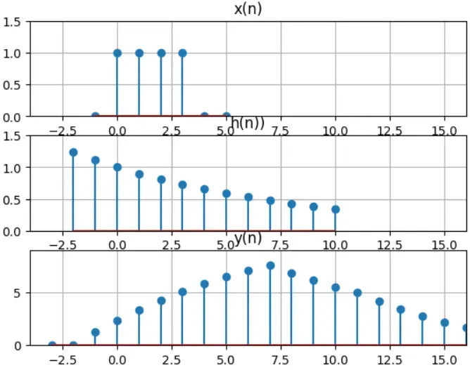

 然后相关序列计算，切记，千万不要和person系数混淆了，我先用person那个函数计算来着，后来发现是不对的，signal.correlate和np.correlate都可以完成相关计算：

#计算自相关和互相关
import matplotlib.pyplot as plt
import numpy as np
from scipy import signal
from scipy.stats import pearsonr
x=np.array([1,3,5,7,9,11,13,15,17,19])
y=np.array([1,1,1,1,2,2,2,2,2,2])
# 计算自相关函数
auto_corr = signal.correlate(x, x, mode='same')
# 计算互相关函数
cross_corr = signal.correlate(x, y, mode='same')
# np.correlate
print("自相关函数：", auto_corr)
print("互相关函数：", cross_corr)

这里就不放图了，没啥意思，就两个类似山峰的曲线，

16、产生信号波形：

from scipy import signal as signal
t=np.linspace(0,1,200,dtype=float)

# scipy.signal.chirp(t, f0, t1, f1, method='linear', phi=0, vertex_zero=True)

h=signal.chirp(t,0,1,120,method='linear',phi=np.pi/3)#linear线性\quadratic二次扫描、logarithmic对数扫描（这时候f0、f1均不能为零）
plt.plot(t,h)
plt.grid(visible=True)
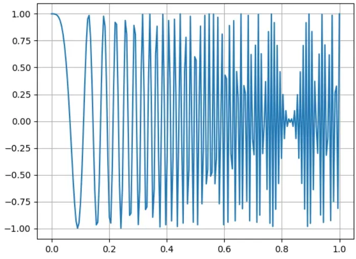
plt.show()

我们这里用singal的chirp函数来生成波形，这里，产生的波形是时间轴为t，时刻0的瞬间频率是f0，时刻t1的瞬间频率是f1，method就是你可以产生波形的方法，phi就是相位，一般来说vertex_zero设置成缺省值就行。

来看一下：

 17、连续矩形周期信号采样变成离散信号：

import matplotlib.pyplot as plt
import numpy as np
from scipy import signal
f=6000
nt=3
N=15
T=1/f
dt=T/N
n=np.linspace(0,50,51,dtype=int)
tn=n*dt
x=signal.square(2*f*np.pi*tn,duty=0.25)+1
fig=plt.figure()
ax1=fig.add_subplot(2,1,1)
ax1.step(tn,x,'k')
ax1.axis([0,nt*T,1.2*min(x),1.1*max(x)])
ax1.set_ylabel('x(t)')
ax2=fig.add_subplot(2,1,2)
ax2.stem(tn,x,'r')
ax2.axis([0,nt*T,1.2*min(x),1.1*max(x)])
ax2.set_ylabel('x(n)')
plt.show()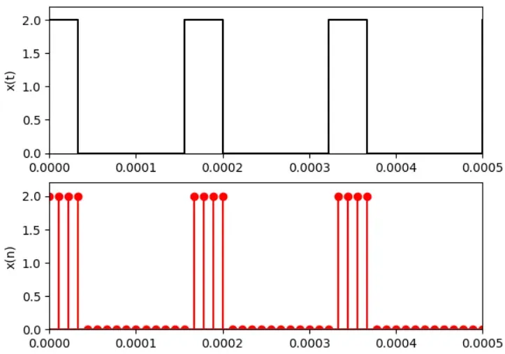

 18、随机函数，这个用numpy就可以直接生成：

#生成随机函数：
t=np.linspace(0,49,dtype=int)
N=len(t)
x=np.random.random(len(t))
fig2=plt.figure()
ax1=fig2.add_subplot(2,1,1)
ax1.plot(t,x)
ax1.set_xlabel('n')
ax1.set_ylabel('x(n)')
ax2=fig2.add_subplot(2,1,2)
ax2.stem(t,x)
ax2.set_xlabel('n')
ax2.set_ylabel('x(n)')
plt.show()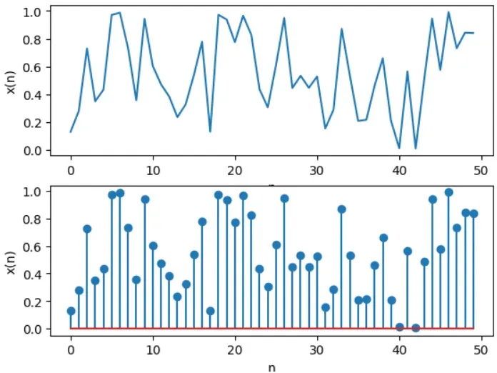

 19、三角波，用signal的sawtooth：

#生成三角波
fs=10000
t=np.linspace(0,1,fs,dtype=float)
x1=signal.sawtooth(1*np.pi*40*t,0)
x2=signal.sawtooth(1*np.pi*40*t,1)
fig3=plt.figure()
ax1=fig3.add_subplot(2,1,1)
ax1.plot(t,x1)
ax1.set_xlabel('n')
ax1.set_ylabel('x(n)')
ax1.axis([0,0.25,-1,1])
ax2=fig3.add_subplot(2,1,2)
ax2.plot(t,x2)
ax2.set_xlabel('n')
ax2.set_ylabel('x(n)')
ax2.axis([0,0.25,-1,1])
plt.show()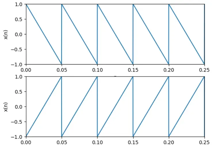

 20、sinc曲线:

t=np.linspace(-3*np.pi,4*np.pi,400,dtype=float)
plt.plot(t,np.sinc(t))
plt.show()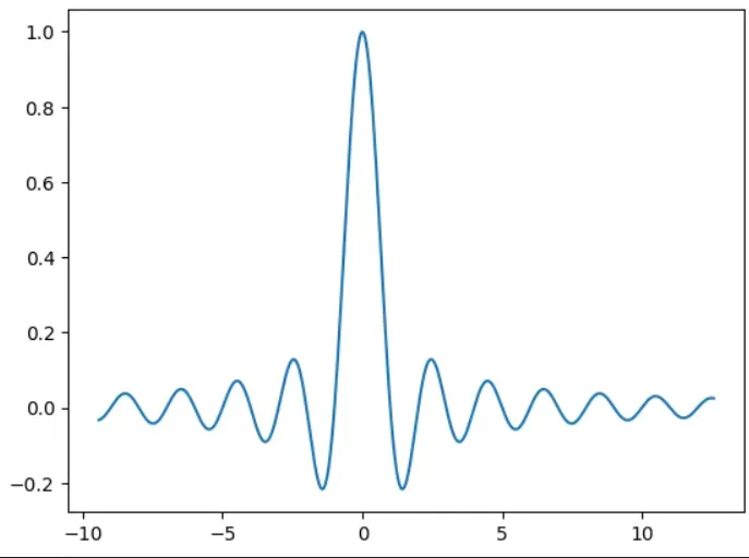

 但是，有一点我到现在还没想通，同样的sinc，用公式推到的和内置的，出来的效果就是不一样：

t=np.linspace(-10,10,10000,dtype=float)
x=np.random.randint(len(t))
y=np.sinc(t)
y1=np.sin(t)
# y2=np.divide(y1,t)
y2=y1/t
fig3=plt.figure()
ax1=fig3.add_subplot(3,1,1)
ax1.plot(t,y)
ax2=fig3.add_subplot(3,1,2)
ax2.plot(t,y1)
ax3=fig3.add_subplot(3,1,3)
ax3.plot(t,y2)
ax3.plot(t,y,'r*')
plt.show()
#好奇怪啊，为什么，已知的是sinc(t)=sin(t)/t，但是我用这种方法做出来的，两个信号的宽度不一样
from mayavi import mlab
from mpl_toolkits.mplot3d import Axes3D
fig=plt.figure()
z=np.linspace(-10,2500,10000,dtype=float).reshape(100,100)
ax=fig.add_subplot(1,1,1, projection='3d')
t2=t.reshape(100,100)
x2=np.sinc(t2)
ax.plot_surface(t2,x2,z,rstride=4,cstride=3,color='r',alpha=0.9)

 三维的我会展示另一幅，以为上面这个代码中的三维太难看了，

import numpy as np
import matplotlib.pyplot as plt
from mpl_toolkits.mplot3d import Axes3D

# 生成数据
x = y = np.linspace(-10, 10, 100)
X, Y = np.meshgrid(x, y)
R = np.sqrt(X**2 + Y**2)
# Z = np.sin(R) / R
z=np.sinc(R)

# 绘制图像
fig = plt.figure()
ax = fig.add_subplot(111, projection='3d')
ax.plot_surface(X, Y, z, cmap='coolwarm')
plt.show()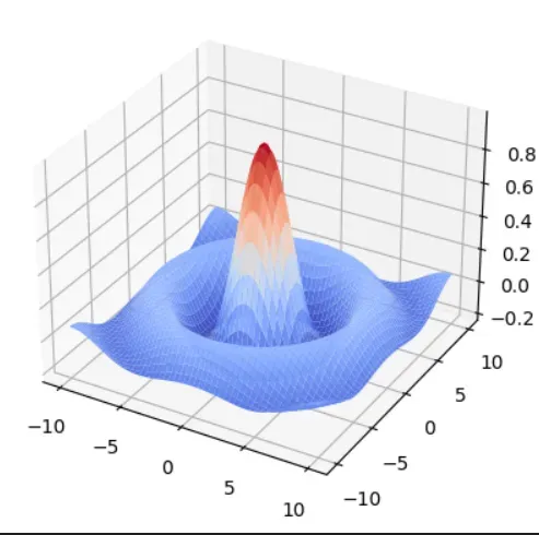

 就这样吧

21、生成非周期三角波

这个利用自己写的函数生成一个就好：

#非周期三角波信号：
t=np.linspace(-2,2,4000)
def triangle_wave(x,c,hc): #幅度为hc，宽度为c,斜度为hc/2c的三角波
    if x>=c/2:
        r=0.0
    elif x<=-c/2:
        r=0.0
    elif((x>-c/2)and(x<0)):
        r=2*x/c*hc+hc
    else:
        r=-2*x/c*hc+hc
    return r
x=np.array([triangle_wave(i,0.5,0.5) for i in t ])
plt.plot(t,x)
plt.show()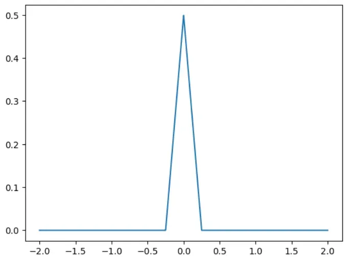

 22、高斯脉冲的实现：

#高斯正弦脉冲：signal.gausspulse(t, fc=1000, bw=0.5, bwr=-6, tpr=-60, retquad=False,retenv=False):
tc=signal.gausspulse('cutoff',60e3,0.6,tpr=-40)
tG=np.linspace(-tc,tc,100000)
y=signal.gausspulse(tG,60e3,0.6)
plt.plot(tG,y)
plt.show()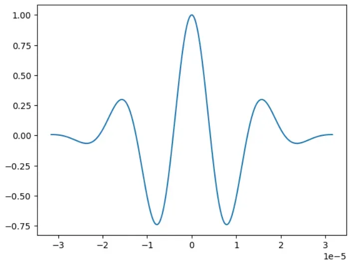

 23、脉冲序列发生器：

这个就是上面的square函数和sawtooth：

import matplotlib.pyplot as plt
import numpy as np
from scipy import signal
n=np.linspace(0,10,dtype=float)
h=signal.square(1*np.pi*40*n)
z=signal.sawtooth(1*np.pi*40*n)
fig=plt.figure()
ax1=fig.add_subplot(2,1,1)
ax1.plot(n,h)
ax1.set_title('square')
ax2=fig.add_subplot(2,1,2)
ax2.plot(n,z)
ax2.set_title('sawtooth')
plt.show()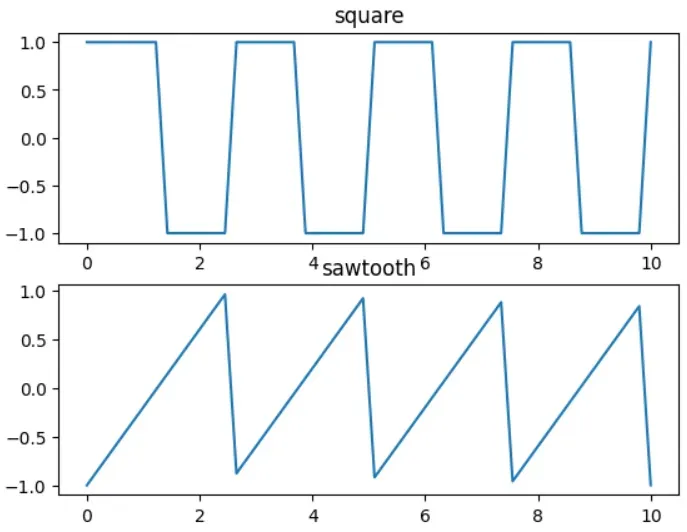

24、产生非周期方波：

#产生非周期方波:matlab 中用的是rectpuls,python似乎还没有这个函数，但是可以自己实现，这是我复制的别人滴
def rect_wave(x,c,c0):     #起点为c0，宽度为c的矩形波
     if x>=(c+c0):
          r=0.0
     elif x<c0:
          r=0.0
     else:
          r=1
     return r

t=np.linspace(-3,3,6000)
y1=np.array([rect_wave(i,1.0,-2.0) for i in t])
plt.plot(t,y1)
plt.show()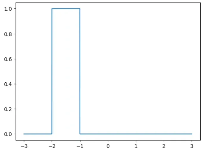

25、连续时间信号的时域分析

（注意，到这里就很注重系统的概念了）

就是求解齐次方程和非齐次方程求解零输入响应和零状态响应：

（1）零状态响应：

#连续时间系统数值求解：matlab有提供函数lsim，python中应该有：scipy包里面有lsim函数：def lsim(system, U, T, X0=None, interp=True):和matlab中的几乎一模一样
from scipy import signal as signal
ts=0
te=5
dt=0.01
# 计算系统的零状态响应,系统是：y''+2y'+100y=10cos(2*pi*t)
# 这里，第一项是右端系数，第二项是左端系数，实际上，lti官方文档给的示例是4个二维矩阵，但我没有明白他们是要干什么。
sys=signal.lti([1],[1,2,200])
t=np.linspace(ts,te,500)
f=10*np.cos(2*np.pi*t)
T,yout,xout=signal.lsim2(sys,f,t)
plt.plot(t,yout)
plt.show()
# 和matlab书上展示的一模一样,展示了该系统的零状态响应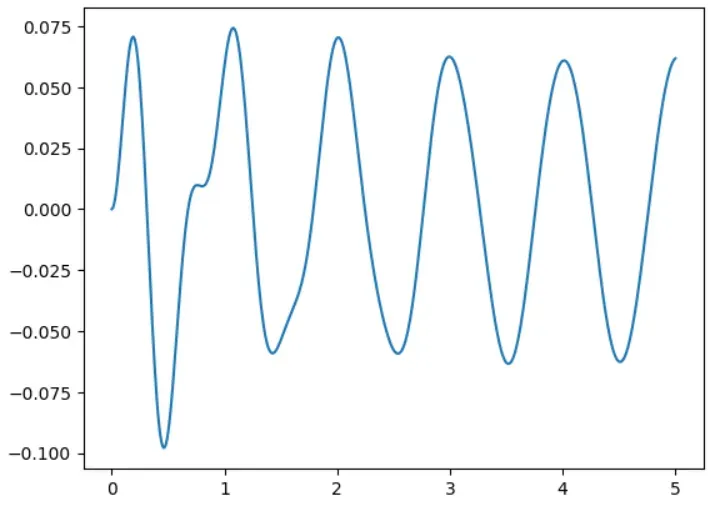

 （2）冲激响应和阶跃响应：

# 连续时间系统系统冲击响应和节约响应：这个matlab有impuls和step，python也当然是有滴，就在singal里面:
import matplotlib.pyplot as plt
import numpy as np
from scipy import signal
t=np.linspace(0,4,2000)
system=([1,32],[1,4,64])
t,h=signal.impulse(system,T=t,N=2000)
t1,g=signal.step(system,T=t,N=2000)
fig1=plt.figure()
ax1=fig1.add_subplot(2,1,1)
ax1.plot(t,h)
ax1.set_xlabel("t")
ax1.set_ylabel('h(t)')
ax1.set_title('impulse')
ax1.grid(visible=True)
ax1.axis([0,4,-1.5,3])
ax2=fig1.add_subplot(2,1,2)
ax2.plot(t1,g)
ax2.set_xlabel("t")
ax2.set_ylabel('g(t)')
ax2.set_title('step')
ax2.grid(visible=True)
ax2.axis([0,4,0,1])
plt.show()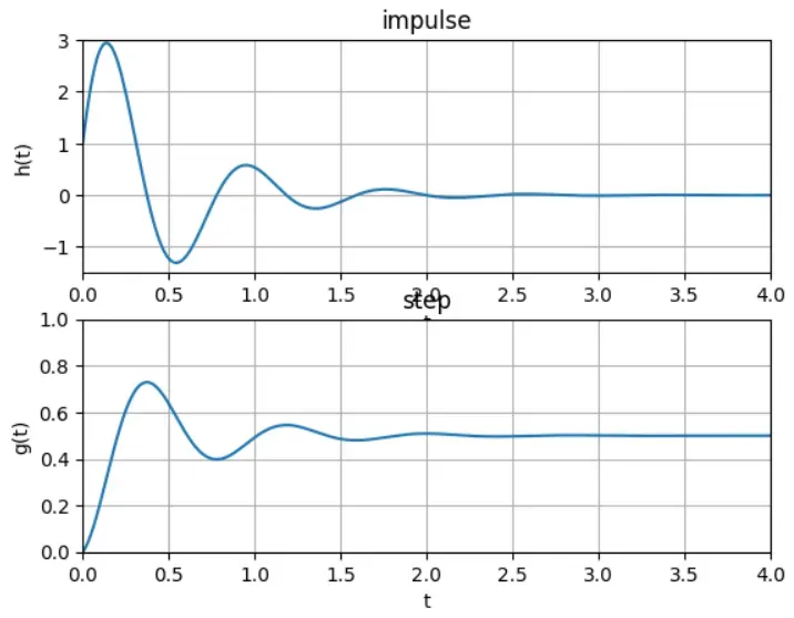

 （3）各种信号的响应：

#计算一个特定系统：
import matplotlib.pyplot as plt
import numpy as np
from scipy import signal

b=[-0.46,-0.25,-0.12,-0.06]
a=[1,0.64,0.94,0.51,0.01]
system=(b,a)
t1=np.linspace(0,10,10000)
t2=np.linspace(-5,5,10000)
f1=np.zeros(len(t1))
def rect_wave(x,c,c0):     #起点为c0，宽度为c的矩形波
     if x>=(c+c0):
          r=0.0
     elif x<c0:
          r=0.0
     else:
          r=1
     return r
def heaviside(x):
     if x==0:
          r=0.5
     elif x>0:
          r=1
     elif x<0:
          r=0
     return r
def unit(t):
    r=np.where(t>0.0,1.0,0.0)
    return r
f1=np.array([heaviside(i)for i in t1])-np.array([heaviside(i) for i in t1])
# f2=np.array([rect_wave(i,1,-1) for i in t2])
f2=np.ones(len(t1))
f2[10:11]=0
f3=t1
f4=np.sin(t1)
T1,yout1,xout1=signal.lsim2(system,f1,t1)
T2,yout2,xout2=signal.lsim2(system,f2,t1)
T3,yout3,xout3=signal.lsim2(system,f3,t1)
T4,yout4,xout4=signal.lsim2(system,f4,t1)
#f1、f2这两个有些问题
fig2=plt.figure()
ax1=fig2.add_subplot(2,2,1)
ax1.plot(t1,yout1)
ax1.set_title('chongji')
ax2=fig2.add_subplot(2,2,2)
ax2.plot(t1,yout2)
ax2.set_title('jump')
ax3=fig2.add_subplot(2,2,3)
ax3.plot(t1,yout3)
ax3.set_title('xiepo')
ax4=fig2.add_subplot(2,2,4)
ax4.plot(t1,yout4)
ax4.set_title('sin')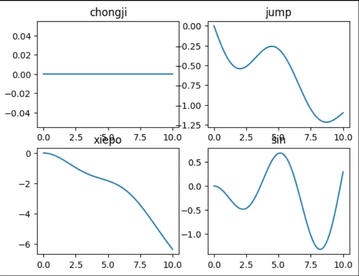

 [0,0]这幅图有些问题，其他的都没啥问题。

（4）连续时间信号的卷积：

#连续时间信号卷积求解：
import matplotlib.pyplot as plt
import numpy as np
from scipy import signal
dt=0.01
t=np.linspace(-1,2.5,350)
t1=t-2
# matlab的heaviside函数是一个阶跃函数，当输入为0时返回0.5，当输入大于0时返回1，当输入小于0时返回0。它的定义是:
# heaviside(x) = 0.5, x = 0
# heaviside(x) = 1, x > 0
# heaviside(x) = 0, x < 0
def heaviside(x):
    if x==0:
          r=0.5
    elif x>0:
          r=1
    elif x<0:
          r=0
    return r
def unit(t):
    r=np.where(t>0.0,1.0,0.0)
    return r
f1=np.array([heaviside(i)for i in t])-np.array([heaviside(i) for i in t1])*0.5
f2=2*np.exp(-3*t)*np.array([heaviside(i)for i in t])
f=np.convolve(f1,f2)*dt
n=len(f)
tt=np.linspace(0,n,n)*dt-2
fig3=plt.figure()
ax1=fig3.add_subplot(3,2,1)
ax1.plot(t,f1)
ax1.axis([-1,2.5,0,1.2])
ax1.set_title('f1(t)')
ax1.grid(visible=True)
ax2=fig3.add_subplot(3,2,2)
ax2.plot(t,f2)
ax2.axis([-1,2.5,0,2])
ax2.set_title('f2(t)')
ax2.grid(visible=True)
ax3=fig3.add_subplot(3,1,2)
ax3.plot(tt,f)
ax3.axis([-2,5,0,1])
ax3.set_title('convolve')
ax3.grid(visible=True)
f4=signal.convolve(f1,f2)*dt
ax4=fig3.add_subplot(3,1,3)
ax4.plot(tt,f4)
ax4.axis([-2,5,0,1])
ax4.set_title('convolve')
ax4.grid(visible=True)
plt.show()

 这里第三张用的是numpy的卷积函数，第四张用的是signal的卷积函数，我就是想看看，两者有没有上面出入。

26、离散时间系统：

实现离散时间系统的实现连续时间系统是很简单的，用numpy就行，说白了，连续就是点很多，很密，就和微分一样，我分的越细，它逼近的就越好，离散也一样，你就认为在和连续时间信号两者范围相同的情况下，区区有限个点就行：

import matplotlib.pyplot as plt
import numpy as np
from scipy import signal
#离散
t=np.linspace(-10,10,41,dtype=float)
#连续
t1=np.linspace(-10,10,10000000,dtype=float)
x=signal.square(np.pi*2*t)
x1=signal.square(np.pi*2*t1)
fig=plt.figure()
ax1=fig.add_subplot(2,1,1)
ax1.stem(t,x)
ax1.set_title('discrete')
ax2=fig.add_subplot(2,1,2)
ax2.plot(t1,x1)
ax2.set_title('coiled')
plt.show()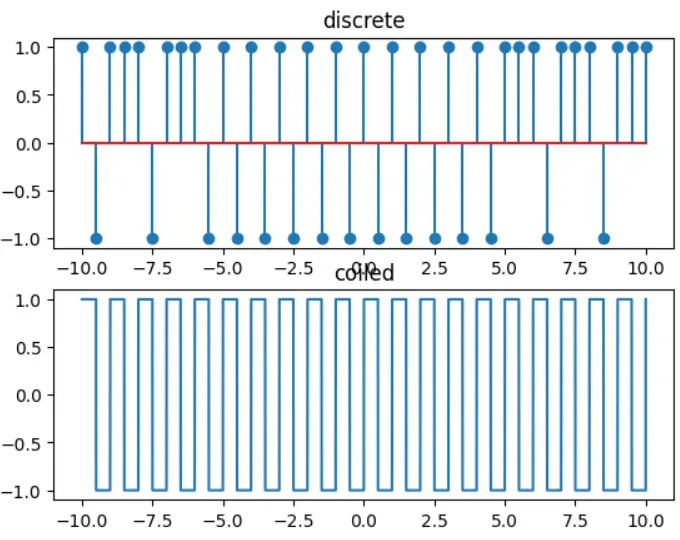

 可以看到，上下两图的区别。

27、离散时间系统的冲激和阶跃响应：

import matplotlib.pyplot as plt
import numpy as np
from scipy import signal
a=[1,-0.35,1.5]
b=[1,1]
system=(b,a)
t=np.linspace(0,21,21,dtype=int)
x=np.power(0.5,t)
T,yout,xout=signal.lsim2(system,T=t)
print(T.size,yout.size,xout.size)
fig1=plt.figure()
ax1=fig1.add_subplot(1,2,1)
ax1.stem(t,x)
ax1.set_title('imput Sequence')
ax1.grid(visible=True)
ax2=fig1.add_subplot(1,2,2)
ax2.stem(t,yout)
ax2.set_title('output Sequence')
ax2.grid(visible=True)
plt.show()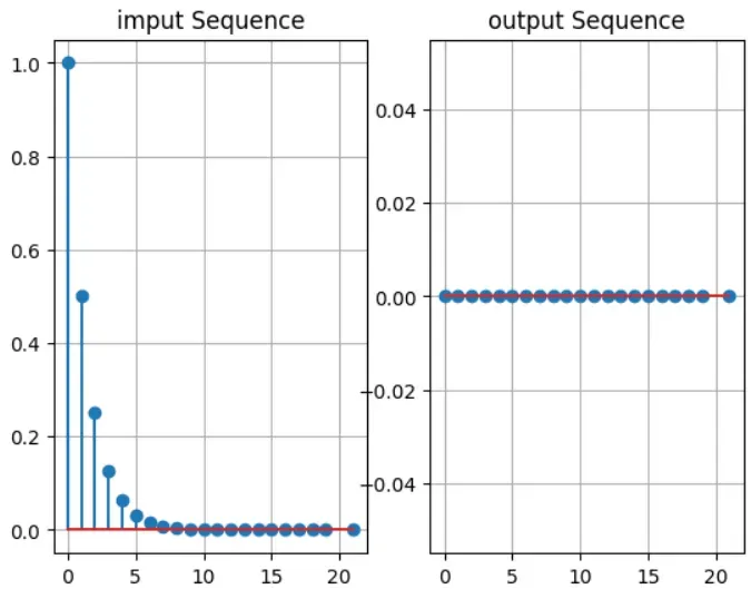

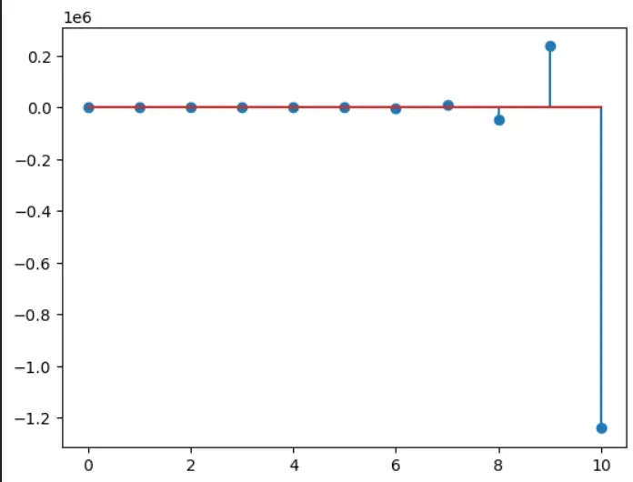
import matplotlib.pyplot as plt
import numpy as np
from scipy import signal
a=[1,6,4]
b=[1,3]
k=np.linspace(0,10,11,dtype=int)
system=signal.dlti(b,a)
T,yout=signal.dstep(system,t=k)
plt.stem(T,np.squeeze(yout))

 28、卷积和运算，这都不用说啥了，前面都说过了：

#离散时间信号的卷积和运算
import matplotlib.pyplot as plt
import numpy as np
from scipy import signal
def uDt(n):
    if n>=0:
        y=1
    else:
        y=0
    return y
nx=np.linspace(-1,5,7,dtype=int,endpoint=True)
nh=np.linspace(-2,10,13,dtype=int,endpoint=True)
nx2=nx-4
nh2=nh-9
x=np.array([uDt(i)for i in nx])-np.array([uDt(i)for i in nx2])
h=np.power(0.9,nh)
h1=np.array([uDt(i)for i in nh])-np.array([uDt(i)for i in nh2])
y=np.convolve(h,h1)
ny1=nx[0]+nh[0]
ny=ny1+np.linspace(0,(len(y)),len(y),dtype=int)
fig=plt.figure()
ax1=fig.add_subplot(3,1,1)
ax1.stem(nx,x)
ax1.grid(visible=True)
ax1.set_title('x(n)')
ax1.axis([-4,16,0,1.5])
ax2=fig.add_subplot(3,1,2)
ax2.stem(nh,h)
ax2.grid(visible=True)
ax2.set_title('h(n))')
ax2.axis([-4,16,0,1.5])
ax3=fig.add_subplot(3,1,3)
ax3.stem(ny,y)
ax3.set_title('y(n)')
ax3.grid(visible=True)
ax3.axis([-4,16,0,9])
plt.show()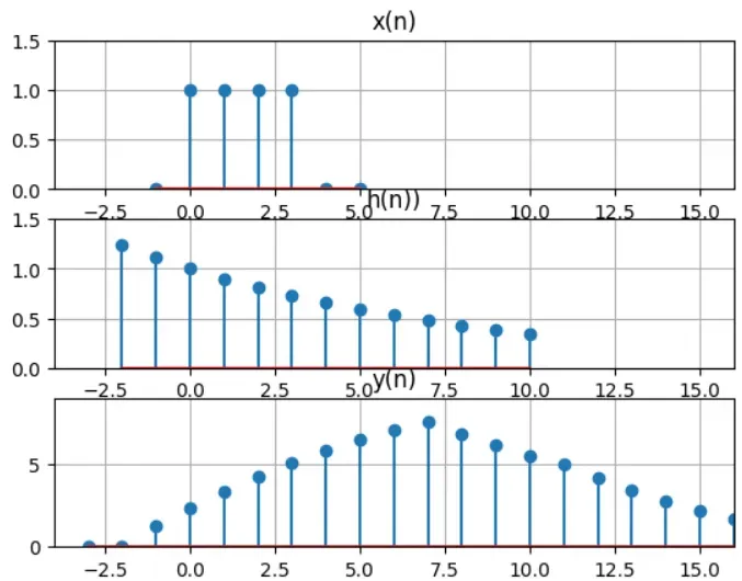

#已知序列卷积求和：
import matplotlib.pyplot as plt
import numpy as np
from scipy import signal
from scipy.stats import pearsonr
x=np.array([1,3,5,7,9,11,13,15,17,19])
y=np.array([1,1,1,1,2,2,2,2,2,2])
z=np.convolve(x,y)
xlength=np.linspace(0,len(x),len(x),dtype=int)
ylength=np.linspace(0,len(y),len(y),dtype=int)
zlength=np.linspace(0,len(z),len(z),dtype=int)
figure=plt.figure()
ax1=figure.add_subplot(3,1,1)
ax1.stem(xlength,x)
ax1.set_title('x(n)')
ax1.grid(visible=True)
ax1.axis([0,len(x),0,20])
ax2=figure.add_subplot(3,1,2)
ax2.stem(ylength,y)
ax2.set_title('y(n)')
ax2.grid(visible=True)
ax2.axis([0,len(y),0,2.2])
ax3=figure.add_subplot(3,1,3)
ax3.stem(zlength,z)
ax3.set_title('z(n)=x(n)*y(n)')
ax3.grid(visible=True)
ax3.axis([0,20,0,max(z)+10])
plt.show()
print(np.corrcoef(x,y))
#这个pearsonr就不用看来，他输出的结果是xy这两个序列的相关系数矩阵，这个在统计学里面会用得到，但现在似乎没有任何用，是我刚开始搞错了
corr_coef, p_value = pearsonr(x, y)
print(corr_coef,p_value)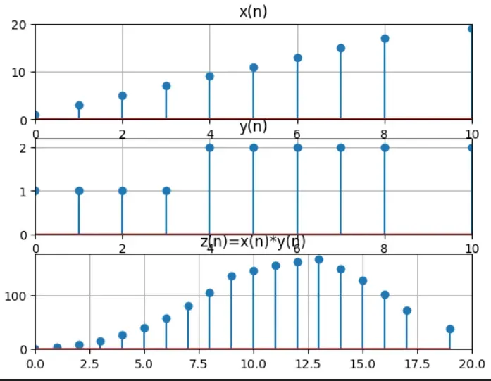

 29、相关序列（自相关、互相关）：

这些前面都讲过了，没啥意思的，这里就不再说了

其实，这两天主要就在忙这个，因为，怎么说呢，我是可以看懂matlab的，但是你要让我去用matlab写代码，我是一百万个不情愿，可能是因为1、我的水平还很低级，2、本科的时候学的是面向对象的C++和Python，对面向对象的编程方式比较熟悉，所以我就选择了使用python来学习数字信号处理，Python很强大，而且都是开源的，对于我来说，Python用起来比Matlab顺手的多，当然，这也是个人原因，办公室的几个师兄师姐就觉得matlab比c++和python简单，所以他们Matlab用的多，但是，说白了，编程语言就是个简单工具，最重要的还是算法和思想。