python复杂网络分析库NetworkX

文章目录

- 1.Networkx简介
- 2.图的类型（Graphs）
- 3.图的创建（Graph Creation）
- 4.图的属性（Graph Reporting）
- 5.图算法（Algorithms）
- 6.图的绘制（Drawing）
- 7.数据结构
- 8.用Networks解决图着色问题
- 9.用Networks解决TSP问题

1.Networkx简介

NetworkX 是一个Python包，用于创建、操作和研究复杂网络的结构和功能。提供以下内容：

图、有向图和多重图的数据结构
许多标准图算法（最短路，最大流等）
网络结构及分析方法
经典图、随机图和合成网络的生成器
…

2.图的类型（Graphs）

NetworkX根据图有无方向和是否多边分别以下4种类

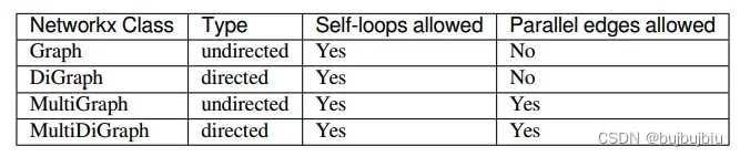
首先根据问题创建你需要的图的实例

import networkx as nx

G = nx.Graph()
G = nx.DiGraph()
G = nx.MultiGraph()
G = nx.MultiDiGraph()

3.图的创建（Graph Creation）

可以用以下三种方法创建NetworkX图对象

图生成器（Graph generators）：创建网络拓扑结构的标准算法
从已经存在的源文件中导入数据
直接添加边和点

直接添加边和顶点是容易描述的

G = nx.Graph()
G.add_edge(1, 2)  # 边(1,2)
G.add_edge(2, 3, weight=0.9)  # 加权边(2,3),权值0.9

边的属性可多样

import math
G.add_edge('y', 'x', function=math.cos)
G.add_node(math.cos)  # 任何可哈希的都可以成为顶点

可以一次添加多条边

elist = [(1, 2), (2, 3), (1, 4), (4, 2)]
G.add_edges_from(elist)
elist = [('a', 'b', 5.0), ('b', 'c', 3.0), ('a', 'c', 1.0), ('c', 'd', 7.3)]
G.add_weighted_edges_from(elist)

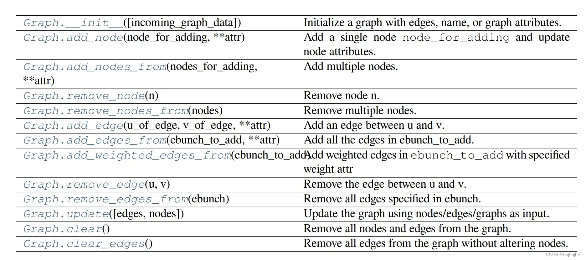
NetworkX添加和移走点和边的方法如下：

4.图的属性（Graph Reporting）

对于一个图，通常需要查看的视图信息包括：顶点，边，邻接点，度。这些视图提供对属性的迭代，数据属性查找等。视图引用图形数据结构，因此任何更改都会显示在视图里。常用属性有：

G.edges代表所有边

for e in list(G.edges):
    print(e)
    
(1, 2)
(1, 4)
(2, 3)
(2, 4)
('y', 'x')
('a', 'b')
('a', 'c')
('b', 'c')
('c', 'd')

G.edges.items()和G.edges.values()和python中的字典功能相似，

for e, datadict in G.edges.items():
    print(e, datadict)
    
(1, 2) {}
(1, 4) {}
(2, 3) {'weight': 0.9}
(2, 4) {}
('y', 'x') {'function': <built-in function cos>}
('a', 'b') {'weight': 5.0}
('a', 'c') {'weight': 1.0}
('b', 'c') {'weight': 3.0}
('c', 'd') {'weight': 7.3}

G.edges.data()会提供具体的属性，包括颜色，权值等

G.edges.data()
Out[23]: EdgeDataView([(1, 2, {}), (1, 4, {}), (2, 3, {'weight': 0.9}), (2, 4, {}), ('y', 'x', {'function': <built-in function cos>}), ('a', 'b', {'weight': 5.0}), ('a', 'c', {'weight': 1.0}), ('b', 'c', {'weight': 3.0}), ('c', 'd', {'weight': 7.3})])

如果想要查找某个点的邻接点（边），可以使用G[u]

G['a']
Out[24]: AtlasView({'b': {'weight': 5.0}, 'c': {'weight': 1.0}})

给出以点1作为顶点的三角形数使用nx.triangles()

nx.triangles(G, 1)
Out[25]: 1

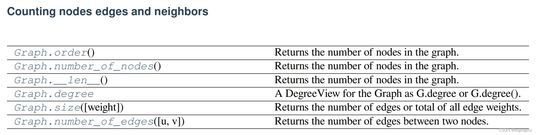
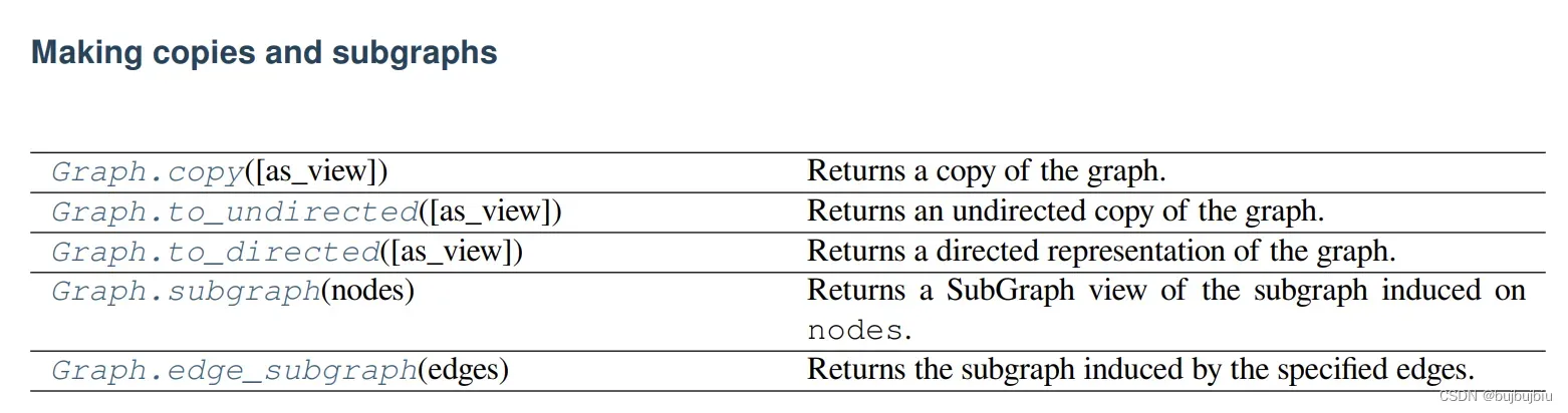
还有许多关于点，边，度的属性使用方法可见networkx_reference

5.图算法（Algorithms）

NetworkX提供了很多图算法，如最短路，广度优先搜索，聚类，同构算法等。例如使用Dijkstra找到最短路

G = nx.Graph()
e = [('a', 'b', 0.3), ('b', 'c', 0.9), ('a', 'c', 0.5), ('c', 'd', 1.2)]
G.add_weighted_edges_from(e)
nx.dijkstra_path(G, 'a', 'd')
Out[30]: ['a', 'c', 'd']

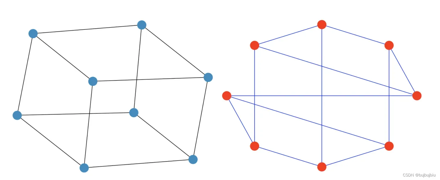
6.图的绘制（Drawing）

NetworkX本身没有绘图工具，但是提供了接口，可以使用其它绘图包Matplotlib等。

import matplotlib.pyplot as plt
G = nx.cubical_graph()  # 3-正则图
subax1 = plt.subplot(121)
nx.draw(G)

subax2 = plt.subplot(122)
# circular_layout：Position nodes on a circle.
nx.draw(G, pos=nx.circular_layout(G), node_color='r', edge_color='b')

7.数据结构

NetworkX使用dictionary of dictionaries of dictionaries作为基础的网络数据结构，这适合存储大规模稀疏网络并且能快速查找。键都是顶底，所有G[u]能返回点u的邻接点和边的属性。查看所有的邻接数据结构可以用G.adj，比如for node, nbrsdict in G.adj.items():。n G[u][v]会返回该边的属性，dict-of-dicts-of-dicts的数据结构有以下优势：

使用两次字典查找可以找到和移除边
优于列表：稀疏存储更能快速查找
优于集合：数据可以和边连接
G[u][v]返回边的属性字典
n in G可以测试点n是否在图G中
for nbr in G[n]迭代所有的邻边

下面是一个两条边的无向图例子，G.adj显示邻接关系

G = nx.Graph()
G.add_edge('A', 'B')
G.add_edge('B', 'C')
G.adj
Out[43]: AdjacencyView({'A': {'B': {}}, 'B': {'A': {}, 'C': {}}, 'C': {'B': {}}})

对于DiGraph图，使用两个dict-of-dicts-of-dicts的结构，一个表示后继G.succ，一个表示前者G.pred。对于 MultiGraph/MultiDiGraph使用dict-of-dicts-of-dicts-of-dicts的结构。
获取边的数据属性有两种接口：adjacency and edges。G[u][v]['width']等效于G.edges[u, v]['width']

G = nx.Graph()
G.add_edge(1, 2, color='red', weight=0.84, size=300)
G[1][2]['size']
Out[46]: 300
G.edges[1, 2]['color']
Out[47]: 'red'

8.用Networks解决图着色问题

提供了两种着色方法：

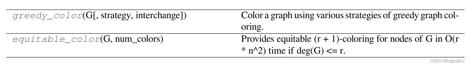
greedy_color(G, strategy='largest_first', interchange=False)：用尽可能少的颜色给图涂色，且相邻点不同色，策略决定了顶点着色的顺序
equitable_color(G, num_colors)：用r种颜色给图着色，相邻不同色，每个颜色的顶点数相差最多1

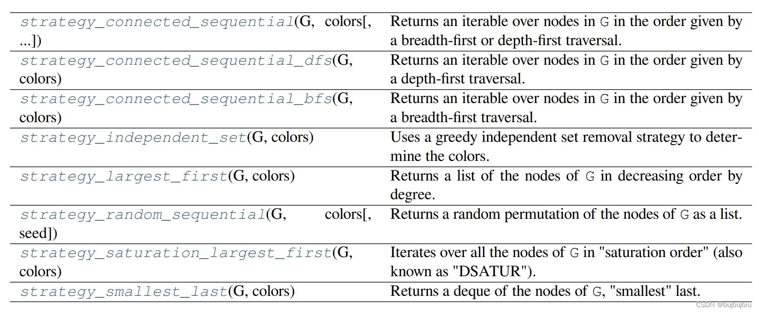
greedy_color()的策略有以下几种：

strategy_connected_sequential_dfs：深度优先遍历
strategy_connected_sequential_bfs：广度优先遍历
strategy_independent_set：找到最大独立集分配颜色后移走
strategy_largest_first：优先选择度最高的点
strategy_saturation_largest_first：饱和度算法，顶点的饱和度定义为当前分配给相邻顶点的不同颜色的数量
strategy_smallest_last：优先选择度最小的点

G = nx.cycle_graph(4)
nx.coloring.greedy_color(G, strategy="largest_first")
Out[49]: {0: 0, 1: 1, 2: 0, 3: 1}

nx.coloring.equitable_color(G, num_colors=3)
Out[54]: {0: 2, 1: 1, 2: 2, 3: 0}

9.用Networks解决TSP问题

traveling_salesman_problem(G, weight='weight', nodes=None, cycle=True, method=None)[source]

 - G：NetworkX graph，可以是加权网络
 - nodes：必须经过的点集合，默认是G.nodes，即哈密尔顿回路
 - weight：边权重，默认为1
 - cycle：是否返回cycle
 - method：TSP算法，有向图默认是threshold_accepting_tsp()，无向图默认是christofides()

import networkx as nx
tsp = nx.approximation.traveling_salesman_problem
G = nx.cycle_graph(9)
G[4][5]['weight'] = 5
tsp(G, nodes=[3, 6])  # 回路从3出发，经过6，回到3

Out[8]: [3, 2, 1, 0, 8, 7, 6, 7, 8, 0, 1, 2, 3]

tsp(G)  # 经过所有顶点一次回到原点
Out[10]: [0, 8, 7, 6, 5, 4, 3, 2, 1, 0]

提供的TSP算法如下：

christofides
greedy_tsp
simulated_annealing_tsp
threshold_accepting_tsp
asadpour_atsp

可以自己构建函数调用这些TSP算法，如使用元启发式模拟退火方法

SA_tsp = nx.approximation.simulated_annealing_tsp
method = lambda G, wt:SA_tsp(G, 'greedy', weight=wt, temp=500)
tsp(G, method=method)
Out[13]: [0, 1, 2, 3, 4, 5, 6, 7, 8, 0]

文章出处登录后可见！

已经登录？立即刷新