目录
前言
一、padim算法onnx模型输入输出解读
二、padim算法Python代码处理流程分析
2.1 预处理部分
2.2 预测部分
2.3 后处理部分
2.4 可视化部分
三、总结与展望
前言
上一篇博客中完成了Anomalib中padim算法的模型训练,得到了onnx模型以及推理的效果,想看这部分的同学可以上翻…对于像我一样根本没读论文的同学,获得了onnx模型以后大概率一脸懵,输入是什么?输出是什么?需要经过什么样的预处理和后处理?如何画出和Anomalib项目中一样好看的概率热图呢?C++中如何部署?本篇博客会带大家逐个分析这些问题。本来想和C++部署一起写的,但是实在太长了。想直接看C++代码的同学略过本篇(不过还是建议看一下),下一篇三天内发出来Orz…
一、padim算法onnx模型输入输出解读
当我们不知道模型里面的结构时,借助Netron工具往往是比较好的办法,Netron网站地址:
Netronhttps://netron.app/ 将模型拖入,界面上就会显示网络结构,以下是padim的onnx模型的输入和输出部分的结构:
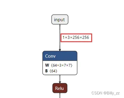
可以看出,其输入尺寸是1*3*256*256,熟悉深度学习的同学应该知道这是一个张量(Tensor),它来源于一张3通道RGB图像,其长宽均为256像素。
结论1:输入是预处理后的256*256的RGB图像。
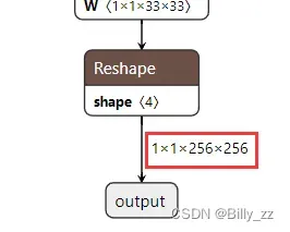
输出也是一个张量,只不过其尺寸为1*1*256*256,见到和原图长宽尺寸相等的数据,我们可以大胆猜测:输出就是我们想要的概率热图,或者某种每个像素位置的得分图,只不过不一定是最终形式。
结论2:输出是某种得分图,经过后处理后也许可以得到概率热图。
总的来说,这个模型的输入和输出并不复杂,这对我们进行算法部署是一件好事。
二、padim算法Python代码处理流程分析
我们虽然急于脱离开Anomalib这个复杂的项目环境,投入下一步的C++部署。但在此之前,我们必须把Python代码运行全过程搞明白,才有可能完成C++的改写。这个过程包括预处理、推理、后处理和可视化四部分。
由于使用了onnx模型进行推理,根据官网教程,此处应该使用tools/inference/openvino_inference.py进行推理。打开该py文件,很容易在infer函数中找到以下代码段:
    for filename in filenames:
        image = read_image(filename, (256, 256))
        predictions = inferencer.predict(image=image)
        output = visualizer.visualize_image(predictions)
这几行代码就是我们探究推理过程的根源。首先使用read_image读入图片,然后调用inferencer的predict方法得到推理结果,最后使用visualizer将推理结果可视化。以上就是使用C++部署时要还原的过程。
read_image比较简单,大家可以自行阅读源码。这里从inferencer开始看起。这里的inferencer由OpenVINOInferencer实例化而来,阅读其predict方法,可以找到如下代码:
        processed_image = self.pre_process(image_arr)              # 预处理
        predictions = self.forward(processed_image)                # 预测
        output = self.post_process(predictions, metadata=metadata) # 后处理

        return ImageResult(
            image=image_arr,
            pred_score=output["pred_score"],
            pred_label=output["pred_label"],
            anomaly_map=output["anomaly_map"],
            pred_mask=output["pred_mask"],
            pred_boxes=output["pred_boxes"],
            box_labels=output["box_labels"],                       # 返回的各项参数
可以看到,图像经过了预处理、预测和后处理之后得到了output结果(字典),返回值为各项参数。根据返回值各项参数的名称,我们可以知道该函数返回了预测的得分、标签类别、异常图等等。
2.1 预处理部分
首先看pre_process部分,在openvino_inferencer.py中定义了该方法:
    def pre_process(self, image: np.ndarray) -> np.ndarray:
        """Pre process the input image by applying transformations.

        Args:
            image (np.ndarray): Input image.

        Returns:
            np.ndarray: pre-processed image.
        """
        transform = A.from_dict(self.metadata["transform"])
        processed_image = transform(image=image)["image"]

        if len(processed_image.shape) == 3:
            processed_image = np.expand_dims(processed_image, axis=0)

        if processed_image.shape[-1] == 3:
            processed_image = processed_image.transpose(0, 3, 1, 2)

        return processed_image
该方法的核心在于transform,通过查看metadata部分代码,可以认为图片经过了与ImageNet相同的标准化预处理,即RGB的均值为[0.406, 0.456, 0.485],方差为[0.225, 0.224, 0.229]。标准化后需要将其尺寸按照Python代码所示进行修改。
结论3:预处理步骤包括按照ImageNet标准化处理图像,和处理图像的尺寸。
2.2 预测部分
其次看forward部分,就在pre_process部分下方:
    def forward(self, image: np.ndarray) -> np.ndarray:
        """Forward-Pass input tensor to the model.

        Args:
            image (np.ndarray): Input tensor.

        Returns:
            np.ndarray: Output predictions.
        """
return self.network.infer(inputs={self.input_blob: image})这部分就是将经过了pre_process的图像送入模型进行预测,很好理解。上篇博客说过此处不纠结神经网络内部的原理,只需要将其当作黑盒使用即可。经过调试查看,发现其输出确实为与原图尺寸相等的得分图,代表了每个像素位置的分数,分数越高越有可能是异常区域。
2.3 后处理部分
然后是后处理部分,这部分是四部分中最复杂的。
    def post_process(self, predictions: np.ndarray, metadata: dict | DictConfig | None = None) -> dict[str, Any]:
        """Post process the output predictions.

        Args:
            predictions (np.ndarray): Raw output predicted by the model.
            metadata (Dict, optional): Meta data. Post-processing step sometimes requires
                additional meta data such as image shape. This variable comprises such info.
                Defaults to None.

        Returns:
            dict[str, Any]: Post processed prediction results.
        """
        if metadata is None:
            metadata = self.metadata

        predictions = predictions[self.output_blob]

        # Initialize the result variables.
        anomaly_map: np.ndarray | None = None
        pred_label: float | None = None
        pred_mask: float | None = None

        # If predictions returns a single value, this means that the task is
        # classification, and the value is the classification prediction score.
        if len(predictions.shape) == 1:
            task = TaskType.CLASSIFICATION
            pred_score = predictions
        else:
            task = TaskType.SEGMENTATION
            anomaly_map = predictions.squeeze()
            pred_score = anomaly_map.reshape(-1).max()

        # Common practice in anomaly detection is to assign anomalous
        # label to the prediction if the prediction score is greater
        # than the image threshold.
        if "image_threshold" in metadata:
            pred_label = pred_score >= metadata["image_threshold"]

        if task == TaskType.CLASSIFICATION:
            _, pred_score = self._normalize(pred_scores=pred_score, metadata=metadata)
        elif task in (TaskType.SEGMENTATION, TaskType.DETECTION):
            if "pixel_threshold" in metadata:
                pred_mask = (anomaly_map >= metadata["pixel_threshold"]).astype(np.uint8)

            anomaly_map, pred_score = self._normalize(
                pred_scores=pred_score, anomaly_maps=anomaly_map, metadata=metadata
            )
            assert anomaly_map is not None

            if "image_shape" in metadata and anomaly_map.shape != metadata["image_shape"]:
                image_height = metadata["image_shape"][0]
                image_width = metadata["image_shape"][1]
                anomaly_map = cv2.resize(anomaly_map, (image_width, image_height))

                if pred_mask is not None:
                    pred_mask = cv2.resize(pred_mask, (image_width, image_height))
        else:
            raise ValueError(f"Unknown task type: {task}")

        if self.task == TaskType.DETECTION:
            pred_boxes = self._get_boxes(pred_mask)
            box_labels = np.ones(pred_boxes.shape[0])
        else:
            pred_boxes = None
            box_labels = None

        return {
            "anomaly_map": anomaly_map,
            "pred_label": pred_label,
            "pred_score": pred_score,
            "pred_mask": pred_mask,
            "pred_boxes": pred_boxes,
            "box_labels": box_labels,
        }
上篇博客提到,由于我们使用自制数据集,所以task为classification,所以一切TaskType为SEGMETATION和DETECTION的代码段都不用管。本部分的代码可以精简很多:
    def post_process(self, predictions: np.ndarray, metadata: dict | DictConfig | None = None) -> dict[str, Any]:
        """Post process the output predictions.

        Args:
            predictions (np.ndarray): Raw output predicted by the model.
            metadata (Dict, optional): Meta data. Post-processing step sometimes requires
                additional meta data such as image shape. This variable comprises such info.
                Defaults to None.

        Returns:
            dict[str, Any]: Post processed prediction results.
        """
        if metadata is None:
            metadata = self.metadata

        predictions = predictions[self.output_blob]

        # Initialize the result variables.
        anomaly_map: np.ndarray | None = None
        pred_label: float | None = None
        pred_mask: float | None = None

        # If predictions returns a single value, this means that the task is
        # classification, and the value is the classification prediction score.
        if len(predictions.shape) == 1:
            task = TaskType.CLASSIFICATION
            pred_score = predictions

        # Common practice in anomaly detection is to assign anomalous
        # label to the prediction if the prediction score is greater
        # than the image threshold.
        if "image_threshold" in metadata:
            pred_label = pred_score >= metadata["image_threshold"]

        if task == TaskType.CLASSIFICATION:
            _, pred_score = self._normalize(pred_scores=pred_score, metadata=metadata)

        pred_boxes = None
        box_labels = None

        return {
            "anomaly_map": anomaly_map,
            "pred_label": pred_label,
            "pred_score": pred_score,
            "pred_mask": pred_mask,
            "pred_boxes": pred_boxes,
            "box_labels": box_labels,
        }
阅读源码,发现本部分有意义的输出只有pred_score,真正的处理步骤只有一行:
_, pred_score = self._normalize(pred_scores=pred_score, metadata=metadata)进入_normalize部分,可以看到输入的pred_scores是一个张量。事实上,pred_scores即为和原图尺寸相等的概率得分图。同样,输入的pred_scores也只处理了一步,即:
            pred_scores = normalize_min_max(
                pred_scores,
                metadata["image_threshold"],
                metadata["min"],
                metadata["max"],
            )
再进入normalize_min_max部分,可以看到该函数对pred_scores进行了如下处理:
normalized = ((targets - threshold) / (max_val - min_val)) + 0.5这里的max_val和min_val来源于哪里呢?打开训练结果文件夹results/padim/tube/run/weights/onnx/metadata.json,可以文件末尾看到如下信息(tube是我自己的数据集名字):
    "image_threshold": 13.702226638793945,
    "pixel_threshold": 13.702226638793945,
    "min": 5.296699047088623,
    "max": 22.767864227294922
min即为min_val,max即为max_val,其含义分别为pred_score得分图中的最小值和最大值,image_threshold是计算得到的阈值,得分图中大于该阈值的像素位置我们认为它属于异常区域(缺陷),小于该阈值的区域认为是正常区域。经过这一步标准化以后输出pred_scores。
结论4:后处理部分输入为预测部分得到的得分图,输出为标准化后的pred_scores。
2.4 可视化部分
至此,数据处理部分结束,接下来就是如何将数据以概率热图的方式可视化的问题了。回到openvino_inference.py,可以看到visualizer调用了visualize_image方法对数据结果predictions进行了处理,并使用show方法进行可视化。
    for filename in filenames:
        image = read_image(filename, (256, 256))
        predictions = inferencer.predict(image=image)
        output = visualizer.visualize_image(predictions)

        if args.output is None and args.show is False:
            warnings.warn(
                "Neither output path is provided nor show flag is set. Inferencer will run but return nothing."
            )

        if args.output:
            file_path = generate_output_image_filename(input_path=filename, output_path=args.output)
            visualizer.save(file_path=file_path, image=output)

        # Show the image in case the flag is set by the user.
        if args.show:
            visualizer.show(title="Output Image", image=output)
进入visualize_image方法,我们之前在config.yaml文件中将显示模式设为full,visualize_image方法内使用的是_visualize_full方法。
        if self.mode == "full":
            return self._visualize_full(image_result)
层层递进,进入_visualize_full方法,同上,只需要关注task为CLASSIFICATION的代码段。在_visualize_full方法中,可以看到如下代码:
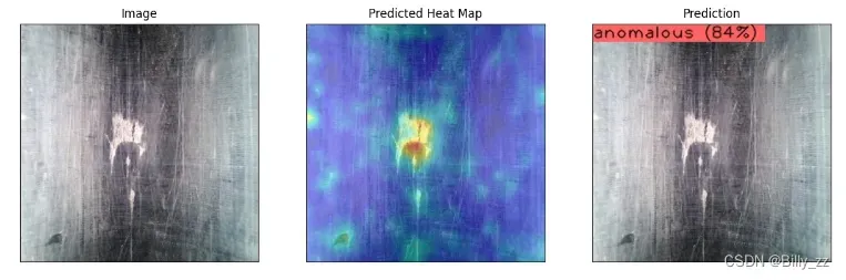
        elif self.task == TaskType.CLASSIFICATION:
            visualization.add_image(image_result.image, title="Image")
            if hasattr(image_result, "heat_map"):
                visualization.add_image(image_result.heat_map, "Predicted Heat Map")
            if image_result.pred_label:
                image_classified = add_anomalous_label(image_result.image, image_result.pred_score)
            else:
                image_classified = add_normal_label(image_result.image, 1 - image_result.pred_score)
            visualization.add_image(image=image_classified, title="Prediction")
visualization.add_image的作用实际上就是往results/padim/tube/run/images的结果中添加图片,添加的三张图片分别为“Image”“Predicted Heat Map”“Prediction”,恰好对应输出的1*3结果图:
这里最关注的还是Predicted Heat Map是怎么画出来的。进入image_result.heat_map,发现它是调用了superimpose_anomaly_map函数生成的:
self.heat_map = superimpose_anomaly_map(self.anomaly_map, self.image, normalize=False)再次进入superimpose_anomaly_map函数,其代码段如下:
def superimpose_anomaly_map(
    anomaly_map: np.ndarray, image: np.ndarray, alpha: float = 0.4, gamma: int = 0, normalize: bool = False
) -> np.ndarray:
    """Superimpose anomaly map on top of in the input image.

    Args:
        anomaly_map (np.ndarray): Anomaly map
        image (np.ndarray): Input image
        alpha (float, optional): Weight to overlay anomaly map
            on the input image. Defaults to 0.4.
        gamma (int, optional): Value to add to the blended image
            to smooth the processing. Defaults to 0. Overall,
            the formula to compute the blended image is
            I' = (alpha*I1 + (1-alpha)*I2) + gamma
        normalize: whether or not the anomaly maps should
            be normalized to image min-max


    Returns:
        np.ndarray: Image with anomaly map superimposed on top of it.
    """

    anomaly_map = anomaly_map_to_color_map(anomaly_map.squeeze(), normalize=normalize)
    superimposed_map = cv2.addWeighted(anomaly_map, alpha, image, (1 - alpha), gamma)
    return superimposed_map
这里的英文注释写的很好了,其实概率热图就是将未处理的原图像和处理后的anomaly_map进行了一定的权重叠加,绘制出的图像。叠加之前,需要对输入的anomaly_map进行anomaly_map_to_color_map函数的处理,而anomaly_map_to_color_map就是将anomaly_map转化为uint8格式的灰度图(像素值0-255),然后根据灰度值绘制伪彩色图:
anomaly_map = cv2.applyColorMap(anomaly_map, cv2.COLORMAP_JET)叠加处理后,一幅清晰明艳的缺陷概率热图就产生了。
结论5:可视化过程中,概率热图为原图和伪彩色anomaly_map的叠加图像。
到这里,我们已经在Python代码的解读中拉通了整个流程:从输入图像到预处理、预测、后处理和可视化,了解了概率热图的绘制方法。
三、总结与展望
若想在C++中部署模型,本篇博客这样耗时又繁琐的代码阅读过程是少不了的。只有先明白原工程中Python代码的逻辑,剥离完整的流程,才可能在C++中进行复现。下一篇博客将以C++代码为主,讲解如何使用OnnxRuntime引擎完成模型的部署。感谢阅读和关注~
文章出处登录后可见!