由系统函数求零极点图、频率响应(幅频特性、相频特性)的 Matlab 和 Python 方法

由系统函数求零极点、频率响应(幅频特性、相频特性)的 Matlab 和 Python 方法

Author: Sijin Yu

文章目录

• 由系统函数求零极点、频率响应(幅频特性、相频特性)的 Matlab 和 Python 方法
• • 1. Matlab
  • • 1.1 tf2zpk() 函数
    • 1.2 zplane() 函数
    • 1.3 freqz() 函数
    • 1.4 Example
  • 2. Python
  • • 2.1 scipy.signal.tf2zpk() 函数
    • 2.2 zplane() 函数的自定义
    • 2.3 scipy.signal.freqz() 函数
    • 2.4 Example
  • 3. 总结

1. Matlab

1.1 tf2zpk() 函数

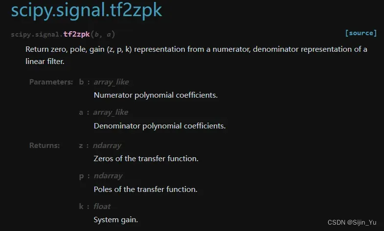
使用 tf2zpk() 函数可以获得频率响应的零极点.
matlab 的官方文档对 tf2zpk() 函数的用法介绍如下.

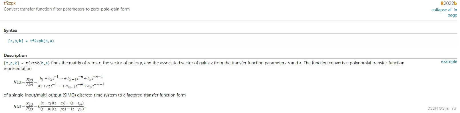
即, 给定系统函数

令序列 . 系统函数的零极点表达式为

序列 分别表示 的零点和极点. 函数 [z, p, k]=tf2zpk(b, a) 返回以 b 和 a 序列为参数的系统方程的零点序列 z、极点序列 p、增益 k.

1.2 zplane() 函数

matlab 的官方文档对 zplane() 函数的用法介绍如下.

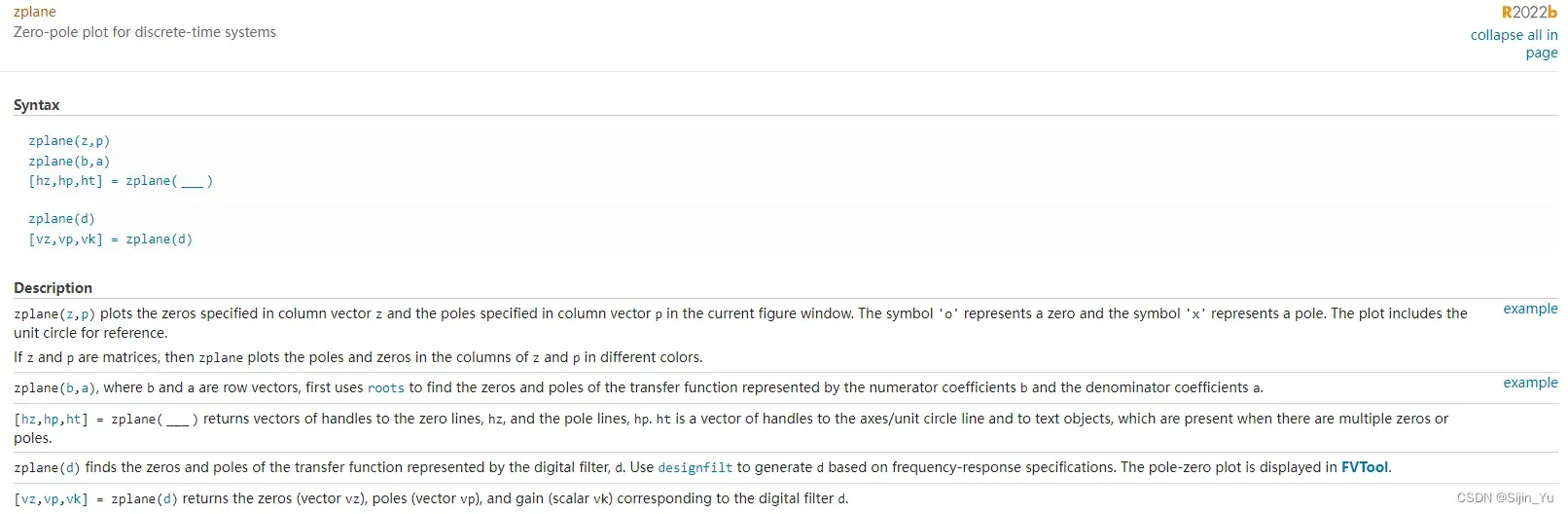
1. zplane(z, p). 传入参数为零点序列 z 和极点序列 p. 直接作零极点图.
2. zplane(b, a). 传入参数为系统函数的参数 b 和 a. 函数自动根据系统函数作零极点图.\

在下文我们会验证这两种做法是等效的.

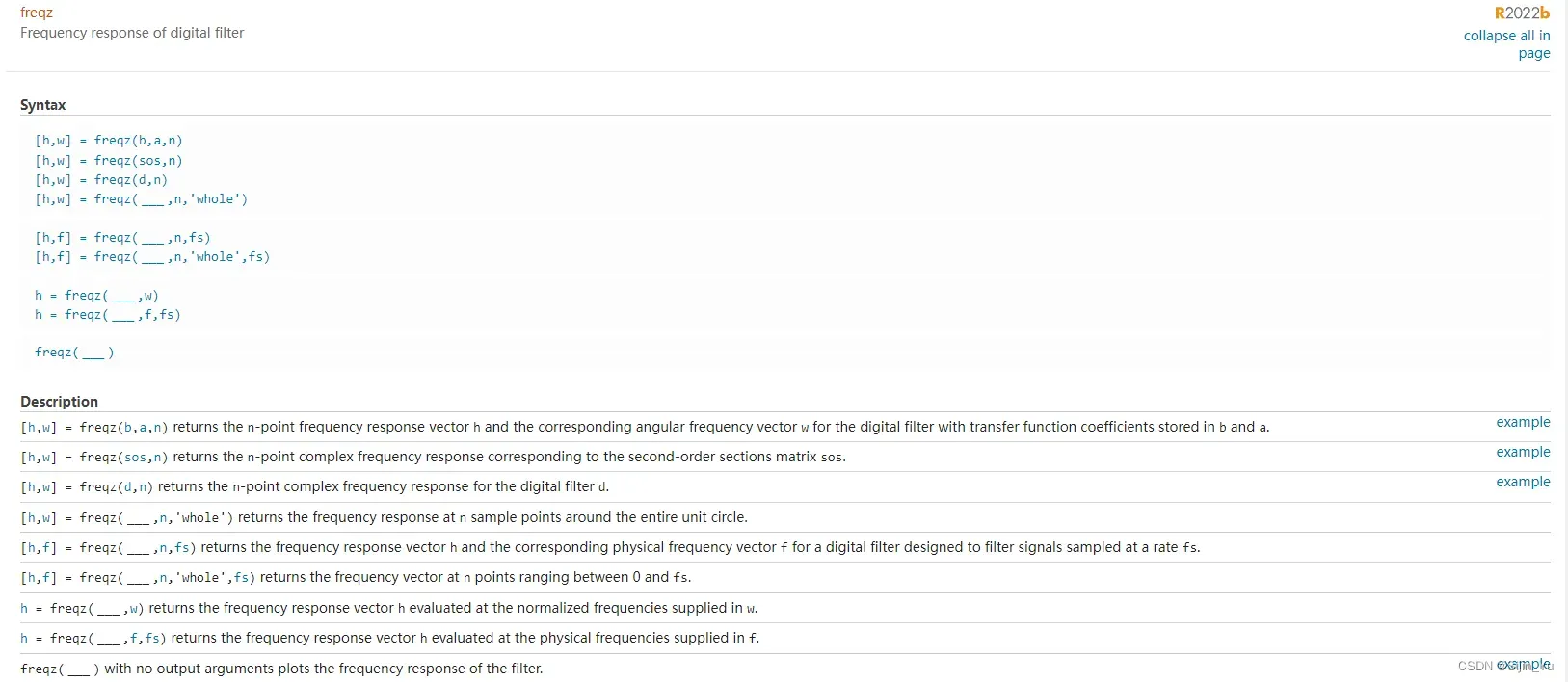
1.3 freqz() 函数

matlab 的官方文档对 freqz() 函数的用法介绍如下.

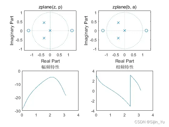
1.4 Example

作下面系统函数的零极点图、幅频特性曲线、相频特性曲线.

代码如下:

% test.m
% author: Sijin Yu
clear;
figure(1);
b = [0 0.5 0 -0.72];
a = [3 2 0.87];
[z, p, k] = tf2zpk(b, a);
% -----零极点----- 
subplot(2, 2, 1);
zplane(z, p);
title('zplane(z, p)');
subplot(2, 2, 2);
zplane(b, a);
title('zplane(b, a)');
% -----幅频特性----- 
[h, w] = freqz(b, a);
H_abs = abs(h);
subplot(2, 2, 3);
plot(w, 20 * log10(H_abs)); % 以分贝为单位
title('幅频特性');
% -----相频特性-----
H_angle = angle(h);
subplot(2, 2, 4);
plot(w, H_angle);
title('相频特性');

结果如下:

2. Python

2.1 scipy.signal.tf2zpk() 函数

该函数依赖 scipy 库, 使用前应执行 pip install scipy.
scipy 的官方文档介绍如下.

2.2 zplane() 函数的自定义

Python 中没有直接实现 matlab 中 zplane() 函数的功能. (至少我没找到, 有知道的大佬欢迎留言.) 因此我自己实现了 zplane() 函数.
函数定义的代码如下

import matplotlib.pyplot as plt
import numpy as np
from matplotlib.patches import Circle

def zplane(z, p, fig=None, ax=None):
    if fig==None or ax==None:
        fig, ax = plt.subplots(figsize=(4, 4))
    circle = Circle(xy = (0.0, 0.0), radius = 1, alpha = 0.9, facecolor = 'white')
    # 作单位园
    theta = np.linspace(0, 2 * np.pi, 200)
    x = np.cos(theta)
    y = np.sin(theta)
    ax.add_patch(circle)
    ax.plot(x, y, color="darkred", linewidth=2)
    lim = max(max(z), max(p), 1) + 1
    # 控制坐标轴范围
    plt.xlim([-lim, lim])
    plt.ylim([-lim, lim])
    # 作零极点
    for i in z:
        ax.plot(np.real(i),np.imag(i), 'bo') 
    for i in p:
        ax.plot(np.real(i),np.imag(i), 'bx') 

2.3 scipy.signal.freqz() 函数

scipy 库官方文档对其描述如下.
(由于内容过长, 不截图)

scipy.signal.freqz(b, a=1, worN=512, whole=False, plot=None, fs=6.283185307179586, include_nyquist=False)

Parameters:

• b: array_like
  Numerator of a linear filter. If b has dimension greater than 1, it is assumed that the coefficients are stored in the first dimension, and b.shape[1:], a.shape[1:], and the shape of the frequencies array must be compatible for broadcasting.
• a: array_like
  Denominator of a linear filter. If b has dimension greater than 1, it is assumed that the coefficients are stored in the first dimension, and b.shape[1:], a.shape[1:], and the shape of the frequencies array must be compatible for broadcasting.
• worN: {None, int, array_like}, optional
  If a single integer, then compute at that many frequencies (default is N=512). This is a convenient alternative to: np.linspace(0, fs if whole else fs/2, N, endpoint=include_nyquist).
  Using a number that is fast for FFT computations can result in faster computations (see Notes).
  If an array_like, compute the response at the frequencies given. These are in the same units as fs.
• whole: bool, optional
  Normally, frequencies are computed from 0 to the Nyquist frequency, fs/2 (upper-half of unit-circle). If whole is True, compute frequencies from 0 to fs. Ignored if worN is array_like.
• plot: callable
  A callable that takes two arguments. If given, the return parameters w and h are passed to plot. Useful for plotting the frequency response inside freqz.
• fs: float, optional
  The sampling frequency of the digital system. Defaults to 2*pi radians/sample (so w is from 0 to pi).
• include_nyquist: bool, optional
  If whole is False and worN is an integer, setting include_nyquist to True will include the last frequency (Nyquist frequency) and is otherwise ignored.

Returns:

• w: ndarray
  The frequencies at which h was computed, in the same units as fs. By default, w is normalized to the range [0, pi) (radians/sample).
• h: ndarray
  The frequency response, as complex numbers.

2.4 Example

我们用回 1.4 中的例子.
代码如下:

# test.py
# author: Sijin Yu
import matplotlib.pyplot as plt
import numpy as np
from scipy import signal
from matplotlib.patches import Circle

def zplane(z, p, fig=None, ax=None):
    if fig==None or ax==None:
        fig, ax = plt.subplots(figsize=(4, 4))
    circle = Circle(xy = (0.0, 0.0), radius = 1, alpha = 0.9, facecolor = 'white')
    # 作单位园
    theta = np.linspace(0, 2 * np.pi, 200)
    x = np.cos(theta)
    y = np.sin(theta)
    ax.add_patch(circle)
    ax.plot(x, y, color="darkred", linewidth=2)
    lim = max(max(z), max(p), 1) + 1
    # 控制坐标轴范围
    plt.xlim([-lim, lim])
    plt.ylim([-lim, lim])
    # 作零极点
    for i in z:
        ax.plot(np.real(i),np.imag(i), 'bo') 
    for i in p:
        ax.plot(np.real(i),np.imag(i), 'bx') 


b = np.array([0, 0.5, 0, -0.72])
a = np.array([3, 2, 0.87])
# -----零极点图-----
z, p, k = signal.tf2zpk(b, a)
fig = plt.figure(figsize=(10, 10))
ax = fig.add_subplot(2, 2, 1)
zplane(z, p, fig=fig, ax=ax)
# -----幅频特性-----
w, h = signal.freqz(b, a)
ax = fig.add_subplot(2, 2, 3)
ax.plot(w, 20 * np.log10(abs(h))) # 以分贝为单位
# -----相频特性-----
ax = fig.add_subplot(2, 2, 4)
ax.plot(w, np.angle(h))
fig.savefig("result_py.jpg")

结果如下:

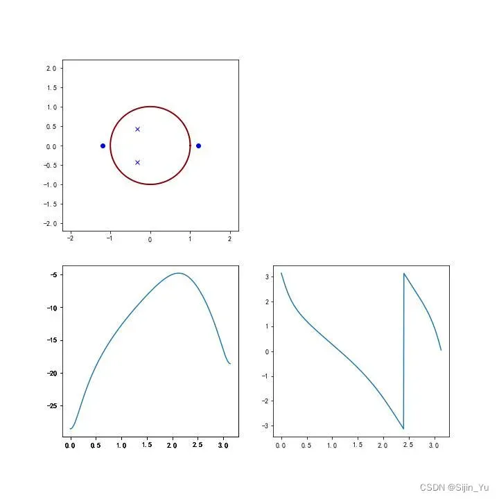
3. 总结

对比 matlab 的图和 Python 的图, 发现为原点的极点 Python 没有画出, 而 matlab 画出. 其余结果 matlab 与 Python 一致.