目录
- 线状堆积图 PolygonPlot
- 三维表面图 SurfacePlot
- 散点图ScatterPlot
- 柱形图 BarPlot
- 三维直方图
- 螺旋曲线图 LinePlot
- ContourPlot
- 轮廓图
- 网状图 WireframePlot
- 箭头图
- 二维三维合并
- 文本图Text
- 三维多个子图
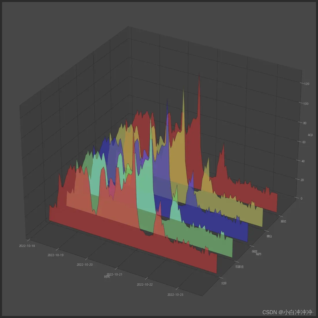
线状堆积图 PolygonPlot
Axes3D.add_collection3d(col, zs=0, zdir=‘z’)
这个函数可以将三维 collection对象或二维collection对象加入到一个图形中,包括:
- PolyCollection
- LineCollection
- PatchCollection
import pandas as pd
from mpl_toolkits.mplot3d import Axes3D
from matplotlib.collections import PolyCollection
import matplotlib.pyplot as plt
from matplotlib import colors as mcolors
import numpy as np
plt.rcParams['font.family'] = 'Microsoft YaHei' # 字体设置
plt.rcParams['font.size'] = 10 # 字体大小设置

fig = plt.figure(figsize=(30,20))
ax = fig.gca(projection='3d')

def cc(arg):
    return mcolors.to_rgba(arg, alpha=0.6)
def polygon_under_graph(xlist, ylist):
    '''
    Construct the vertex list which defines the polygon filling the space under
    the (xlist, ylist) line graph.  Assumes the xs are in ascending order.
    '''
    return [(xlist[0], 0.), *zip(xlist, ylist), (xlist[-1], 0.)]

xs = np.arange(0,137,1)

verts = []

zs = [0.0,1.0,2.0, 3.0,4.0]
for z in zs:
    for i in range(1,6):   #读取数据
        ys = df.iloc[:,i]
    verts.append(polygon_under_graph(xs,ys))

poly = PolyCollection(verts, facecolors=[cc('r'), cc('g'), cc('b'),cc('y'),cc('r')])
poly.set_alpha(0.7)  # 图形的透明度
ax.add_collection3d(poly, zs=zs, zdir='y')

names_1 = ['2022-10-18', '2022-10-19', '2022-10-20','2022-10-21',
'2022-10-22', '2022-10-23']
plt.xticks(xs[::24], names_1)

names = ['北京', '石家庄', '保定','唐山','廊坊']
plt.yticks(zs, names)

ax.set_xlabel('时间')
ax.set_ylabel('城市')
ax.set_zlabel('AQI')
ax.set_xlim3d(0, 136)
ax.set_ylim3d(-1, 5)
ax.set_zlim3d(0, 130)
#plt.savefig('三维时间.png',bbox_inches = 'tight',dpi=500)
plt.show()
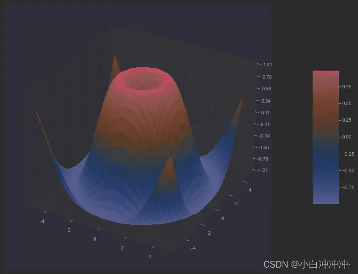
三维表面图 SurfacePlot
Axes3D.plot_surface(X, Y, Z, *args, norm=None, vmin=None, vmax=None, lightsource=None, **kwargs)
这个函数算是比较常用的函数,用于绘制三维表面图,让人惊艳的是它的着色效果。
| Argument | Description |
|---|---|
| X, Y,Z | 坐标点 |
| rcount,ccount,rstride,cstride | 同上 |
| color | 定义surface patch的颜色,type:color-like |
| cmap | 定义surface patch的颜色,只不过是colorMap,type:colormap |
| facecolors | 指定单个patch的颜色, type:array-like of colors |
| norm | colormap的normalization, type:Normalize |
| shade | 阴影效果,type:boolean |
| vmin, vmax | normalization的边界 |
| **kwargs | 向下传递到Poly3DCollection |
| antialiased | 抗锯齿,type:boolean |
from mpl_toolkits.mplot3d import Axes3D
import matplotlib.pyplot as plt
from matplotlib import cm

from matplotlib.ticker import LinearLocator, FormatStrFormatter
import numpy as np


fig = plt.figure(figsize=(30,10))
ax = fig.gca(projection='3d')

# Make data.
X = np.arange(-5, 5, 0.25)
Y = np.arange(-5, 5, 0.25)
X, Y = np.meshgrid(X, Y)
R = np.sqrt(X**2 + Y**2)
Z = np.sin(R)

# Plot the surface.
surf = ax.plot_surface(X, Y, Z, cmap=cm.coolwarm,
                       linewidth=0, antialiased=False)

# Customize the z axis.
ax.set_zlim(-1.01, 1.01)
ax.zaxis.set_major_locator(LinearLocator(10))
ax.zaxis.set_major_formatter(FormatStrFormatter('%.02f'))

# Add a color bar which maps values to colors.
fig.colorbar(surf, shrink=0.5, aspect=5)

plt.show()
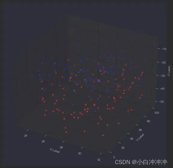
散点图ScatterPlot
Axes3D.scatter(xs, ys, zs=0, zdir=‘z’, s=20, c=None, depthshade=True, *args, **kwargs)
返回Patch3DCollection,
其他参数向下传递给plot函数
| Argument | Description |
|---|---|
| xs, ys | x,y坐标点 |
| zs | z 坐标,可以是一个标量或一个x*y维矩阵,默认是0. |
| zdir | 当绘制二维图像时的z轴方向 |
| s | size,即散点大小 |
| c | 颜色映射,其取值可以是非常多类型,有时间专门写一篇讲解 |
| depthshade | 是否渲染景深(或则就说阴影吧),默认是True. |
from mpl_toolkits.mplot3d import Axes3D

import matplotlib.pyplot as plt
import numpy as np

# Fixing random state for reproducibility
np.random.seed(19680801)

def randrange(n, vmin, vmax):
    '''
    Helper function to make an array of random numbers having shape (n, )
    with each number distributed Uniform(vmin, vmax).
    '''
    return (vmax - vmin)*np.random.rand(n) + vmin

fig = plt.figure(figsize=(20,10))
ax = fig.add_subplot(111, projection='3d')

n = 100

# For each set of style and range settings, plot n random points in the box
# defined by x in [23, 32], y in [0, 100], z in [zlow, zhigh].
for c, m, zlow, zhigh in [('r', 'o', -50, -25), ('b', '^', -30, -5)]:
    xs = randrange(n, 23, 32)
    ys = randrange(n, 0, 100)
    zs = randrange(n, zlow, zhigh)
    ax.scatter(xs, ys, zs, c=c, marker=m)

ax.set_xlabel('X Label')
ax.set_ylabel('Y Label')
ax.set_zlabel('Z Label')

plt.show()
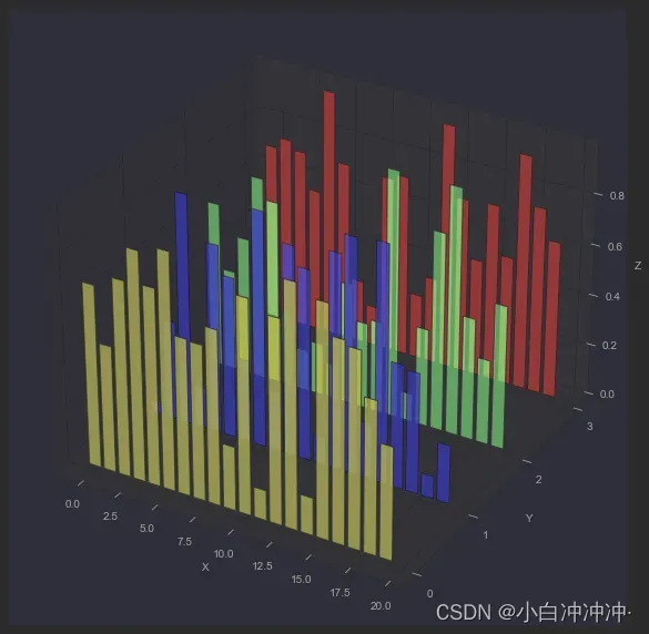
柱形图 BarPlot
Axes3D.bar(left, height, zs=0, zdir=‘z’, *args, **kwargs)
其他参数向下传递给bar函数,返回Patch3DCollection对象
| Argument | Description |
|---|---|
| left | 条形图水平坐标 |
| height | 条形的高度 |
| zs | Z方向 |
| zdir | 同上 |
from mpl_toolkits.mplot3d import Axes3D  # noqa: F401 unused import

import matplotlib.pyplot as plt
import numpy as np

# Fixing random state for reproducibility
np.random.seed(19680801)


fig = plt.figure(figsize=(10,20))
ax = fig.add_subplot(111, projection='3d')

colors = ['r', 'g', 'b', 'y']
yticks = [3, 2, 1, 0]
for c, k in zip(colors, yticks):
    # Generate the random data for the y=k 'layer'.
    xs = np.arange(20)
    ys = np.random.rand(20)

    # You can provide either a single color or an array with the same length as
    # xs and ys. To demonstrate this, we color the first bar of each set cyan.
    cs = [c] * len(xs)

    # Plot the bar graph given by xs and ys on the plane y=k with 80% opacity.
    ax.bar(xs, ys, zs=k, zdir='y', color=cs, alpha=0.8)

ax.set_xlabel('X')
ax.set_ylabel('Y')
ax.set_zlabel('Z')

# On the y axis let's only label the discrete values that we have data for.
ax.set_yticks(yticks)

plt.show()
三维直方图
from mpl_toolkits.mplot3d import Axes3D
import matplotlib.pyplot as plt
import numpy as np

fig = plt.figure()
ax = fig.add_subplot(111, projection='3d')
x, y = np.random.rand(2, 100) * 4
hist, xedges, yedges = np.histogram2d(x, y, bins=4, range=[[0, 4], [0, 4]])

# Construct arrays for the anchor positions of the 16 bars.
# Note: np.meshgrid gives arrays in (ny, nx) so we use 'F' to flatten xpos,
# ypos in column-major order. For numpy >= 1.7, we could instead call meshgrid
# with indexing='ij'.
xpos, ypos = np.meshgrid(xedges[:-1] + 0.25, yedges[:-1] + 0.25)
xpos = xpos.flatten('F')
ypos = ypos.flatten('F')
zpos = np.zeros_like(xpos)

# Construct arrays with the dimensions for the 16 bars.
dx = 0.5 * np.ones_like(zpos)
dy = dx.copy()
dz = hist.flatten()

ax.bar3d(xpos, ypos, zpos, dx, dy, dz, color='b', zsort='average')

plt.show()

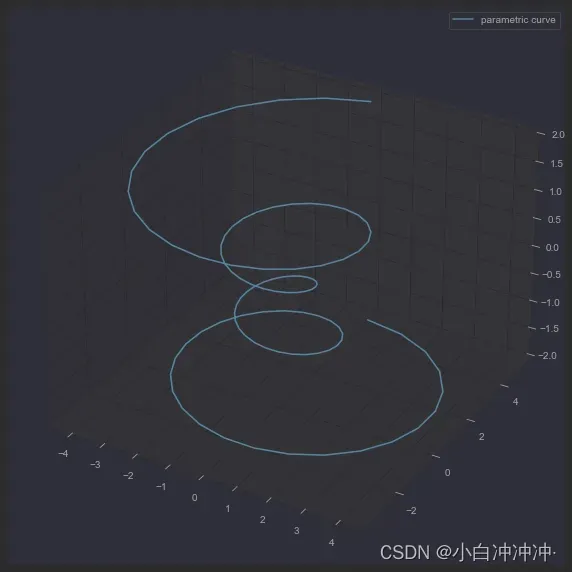
螺旋曲线图 LinePlot
Axes3D.plot(xs, ys, *args, zdir=‘z’, **kwargs)
其他参数向下传递给plot函数
| Argument | Description |
|---|---|
| xs, ys | x、y 坐标 |
| zs | z 坐标,可以是一个标量或一个x*y维矩阵 |
| zdir | 当绘制二维图像时的z轴方向 |
from mpl_toolkits.mplot3d import Axes3D

import numpy as np
import matplotlib.pyplot as plt


plt.rcParams['legend.fontsize'] = 10
fig = plt.figure(figsize=(10,20))
ax = fig.gca(projection='3d')  # get current axes

# Prepare arrays x, y, z
theta = np.linspace(-4 * np.pi, 4 * np.pi, 100)
z = np.linspace(-2, 2, 100)
r = z**2 + 1
x = r * np.sin(theta)
y = r * np.cos(theta)

ax.plot(x, y, z, label='parametric curve')
ax.legend()

plt.show()
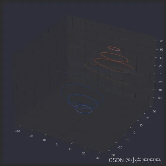
ContourPlot
Axes3D.contour(X, Y, Z, *args, extend3d=False, stride=5, zdir=‘z’, offset=None, **kwargs)
| Argument | Description |
|---|---|
| X, Y,Z | Data values as numpy.arrays |
| extend3d | 是否延申到3d空间 (default: False) |
| *stride | (extend3d的)采样步长 |
| zdir | 同上 |
| offset | 绘制轮廓线在zdir垂直的水平面上的投影 |
from mpl_toolkits.mplot3d import axes3d
import matplotlib.pyplot as plt
from matplotlib import cm

fig = plt.figure(figsize=(30,10))
ax = fig.gca(projection='3d')
X, Y, Z = axes3d.get_test_data(0.05)

# Plot contour curves
cset = ax.contour(X, Y, Z, cmap=cm.coolwarm)

ax.clabel(cset, fontsize=9, inline=1)  # function to label a contour

plt.show()
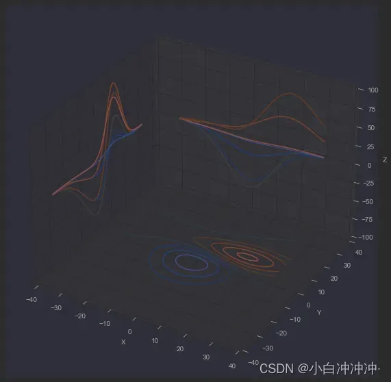
轮廓图
from mpl_toolkits.mplot3d import axes3d
import matplotlib.pyplot as plt
from matplotlib import cm

fig = plt.figure()
ax = fig.gca(projection='3d')
X, Y, Z = axes3d.get_test_data(0.05)
cset = ax.contour(X, Y, Z, zdir='z', offset=-100, cmap=cm.coolwarm)
cset = ax.contour(X, Y, Z, zdir='x', offset=-40, cmap=cm.coolwarm)
cset = ax.contour(X, Y, Z, zdir='y', offset=40, cmap=cm.coolwarm)

ax.set_xlabel('X')
ax.set_xlim(-40, 40)
ax.set_ylabel('Y')
ax.set_ylim(-40, 40)
ax.set_zlabel('Z')
ax.set_zlim(-100, 100)

plt.show()
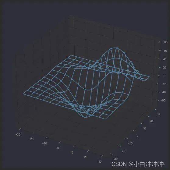
网状图 WireframePlot
Axes3D.plot_wireframe(X, Y, Z, *args, **kwargs)
| Argument | Description |
|---|---|
| X, Y,Z | 坐标点 |
| rcount,ccount | 采样数,越大采样越多,默认50 |
| rstride,cstride | 采样步长,越小采样越多 |
| **kwargs | 其他参数向下传入Line3DCollection |
from mpl_toolkits.mplot3d import axes3d
import matplotlib.pyplot as plt


fig = plt.figure(figsize=(30,10))
ax = fig.add_subplot(111, projection='3d')

# Grab some test data.
X, Y, Z = axes3d.get_test_data(0.05)

# Plot a basic wireframe.
ax.plot_wireframe(X, Y, Z, rstride=10, cstride=10)

plt.show()
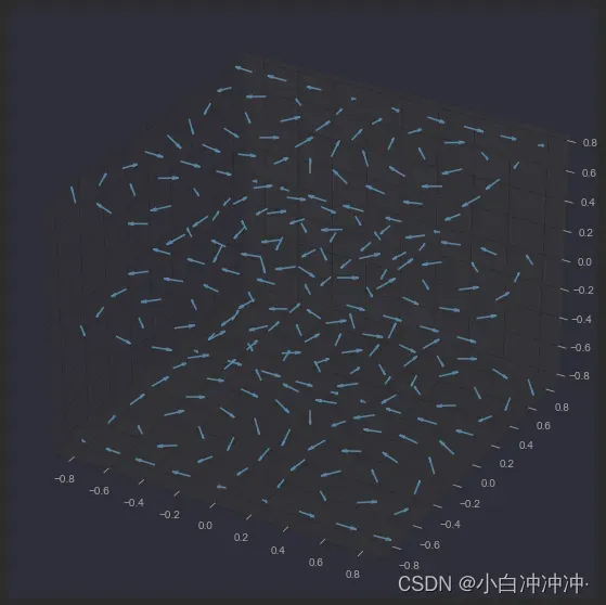
箭头图
Axes3D.quiver(*args, **kwargs)
| Argument | Description |
|---|---|
| X, Y, Z | The x, y and z coordinates of the arrow locations (default is tail of arrow; see pivot kwarg) |
| U, V, W | The x, y and z components of the arrow vectors |
from mpl_toolkits.mplot3d import axes3d
import matplotlib.pyplot as plt
import numpy as np

fig = plt.figure()
ax = fig.gca(projection='3d')

# Make the grid
x, y, z = np.meshgrid(np.arange(-0.8, 1, 0.2),
                      np.arange(-0.8, 1, 0.2),
                      np.arange(-0.8, 1, 0.8))

# Make the direction data for the arrows
u = np.sin(np.pi * x) * np.cos(np.pi * y) * np.cos(np.pi * z)
v = -np.cos(np.pi * x) * np.sin(np.pi * y) * np.cos(np.pi * z)
w = (np.sqrt(2.0 / 3.0) * np.cos(np.pi * x) * np.cos(np.pi * y) *
     np.sin(np.pi * z))

ax.quiver(x, y, z, u, v, w, length=0.1, normalize=True)

plt.show()
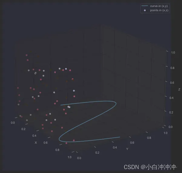
二维三维合并
from mpl_toolkits.mplot3d import Axes3D
import numpy as np
import matplotlib.pyplot as plt

fig = plt.figure()
ax = fig.gca(projection='3d')

# Plot a sin curve using the x and y axes.
x = np.linspace(0, 1, 100)
y = np.sin(x * 2 * np.pi) / 2 + 0.5
ax.plot(x, y, zs=0, zdir='z', label='curve in (x,y)')

# Plot scatterplot data (20 2D points per colour) on the x and z axes.
colors = ('r', 'g', 'b', 'k')
x = np.random.sample(20 * len(colors))
y = np.random.sample(20 * len(colors))
labels = np.random.randint(3, size=80)

# By using zdir='y', the y value of these points is fixed to the zs value 0
# and the (x,y) points are plotted on the x and z axes.
ax.scatter(x, y, zs=0, zdir='y', c=labels, label='points in (x,z)')

# Make legend, set axes limits and labels
ax.legend()
ax.set_xlim(0, 1)
ax.set_ylim(0, 1)
ax.set_zlim(0, 1)
ax.set_xlabel('X')
ax.set_ylabel('Y')
ax.set_zlabel('Z')

# Customize the view angle so it's easier to see that the scatter points lie
# on the plane y=0
ax.view_init(elev=20., azim=-35)

plt.show()
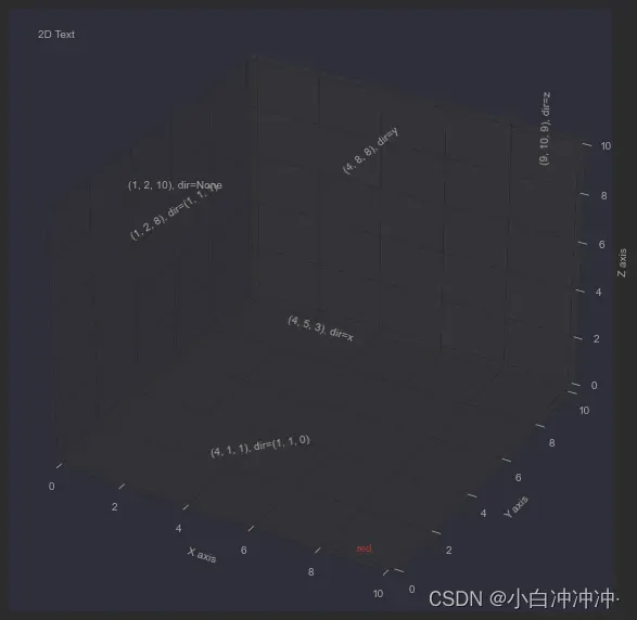
文本图Text
Axes3D.text(x, y, z, s, zdir=None, **kwargs)
text的内容其实也很繁杂,需要用一篇内容去探讨,在三维中很重要的一点是要学会二维、三维文字的添加。
from mpl_toolkits.mplot3d import Axes3D  # noqa: F401 unused import

import matplotlib.pyplot as plt


fig = plt.figure()
ax = fig.gca(projection='3d')

# Demo 1: zdir
zdirs = (None, 'x', 'y', 'z', (1, 1, 0), (1, 1, 1))
xs = (1, 4, 4, 9, 4, 1)
ys = (2, 5, 8, 10, 1, 2)
zs = (10, 3, 8, 9, 1, 8)

for zdir, x, y, z in zip(zdirs, xs, ys, zs):
    label = '(%d, %d, %d), dir=%s' % (x, y, z, zdir)
    ax.text(x, y, z, label, zdir)

# Demo 2: color
ax.text(9, 0, 0, "red", color='red')

# Demo 3: text2D
# Placement 0, 0 would be the bottom left, 1, 1 would be the top right.
ax.text2D(0.05, 0.95, "2D Text", transform=ax.transAxes)

# Tweaking display region and labels
ax.set_xlim(0, 10)
ax.set_ylim(0, 10)
ax.set_zlim(0, 10)
ax.set_xlabel('X axis')
ax.set_ylabel('Y axis')
ax.set_zlabel('Z axis')

plt.show()
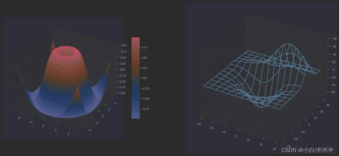
三维多个子图
import matplotlib.pyplot as plt
from mpl_toolkits.mplot3d.axes3d import Axes3D, get_test_data
from matplotlib import cm
import numpy as np

# set up a figure twice as wide as it is tall
# fig = plt.figure(figsize=plt.figaspect(0.5))
fig = plt.figure(figsize=(20,10))

# ===============
#  First subplot
# ===============
# set up the axes for the first plot
ax = fig.add_subplot(1, 2, 1, projection='3d')

# plot a 3D surface like in the example mplot3d/surface3d_demo
X = np.arange(-5, 5, 0.25)
Y = np.arange(-5, 5, 0.25)
X, Y = np.meshgrid(X, Y)
R = np.sqrt(X ** 2 + Y ** 2)
Z = np.sin(R)
surf = ax.plot_surface(X, Y, Z, rstride=1, cstride=1, cmap=cm.coolwarm,
                       linewidth=0, antialiased=False)
ax.set_zlim(-1.01, 1.01)
fig.colorbar(surf, shrink=0.5, aspect=10)

# ===============
# Second subplot
# ===============
# set up the axes for the second plot
ax = fig.add_subplot(1, 2, 2, projection='3d')

# plot a 3D wireframe like in the example mplot3d/wire3d_demo
X, Y, Z = get_test_data(0.05)
ax.plot_wireframe(X, Y, Z, rstride=10, cstride=10)

plt.show()
文章出处登录后可见!