大家好,之前大家对于这篇文章有很多的疑问,包括数据啦,代码啦,所以今天我再次修改一下这篇文章,并且集中解释一下大家的疑惑。
在LDA 的第一步,都是分词,在这里我定义一个方法,
一个对于句子进行分词,并加载停用词与自定义词典。
关于停用词大家可以自己在网上找一份,
import jieba
import jieba.analyse
from pandas.core.frame import DataFrame
from zhon.hanzi import punctuation
from collections import Counter
# jieba.load_userdict('userdict.txt')
# 创建停用词list
import numpy as np
import pandas as pd
def seg_sentence(sentence):
    # 对句子进行分词
    jieba.load_userdict("E:/pythoncode/project/datasets/new/dic/dic.txt") #自定义词典
    sentence_seged = jieba.cut(sentence.strip(), cut_all=False)
    stopwords = stopwordslist('E:/pythoncode/project/datasets/new/dic/CNstopwords.txt')  # 这里加载停用词的路径
    outstr = ''
    for word in sentence_seged:
        if word not in stopwords:
            if word != '\t':
                outstr += word
                outstr += " "
    return outstr
def stopwordslist(filepath):
    # 停用词
    stopwords = [line.strip() for line in open(filepath, 'r', encoding='utf-8').readlines()]
    return stopwords
# 创建一个txt文件,文件名为mytxtfile,并向文件写入msg
然后使用pandas模块读取excel文件,内容格式如下:
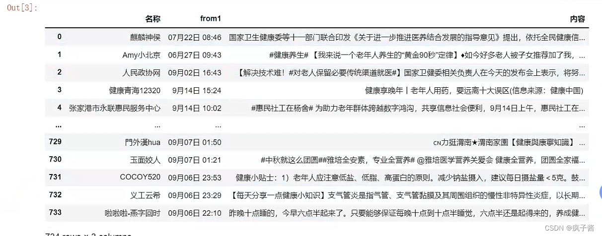
读取后,我们将【“内容”】列转化为列表,并利用jieba进行分词,并且形成新的分词后列表fenci_out, 再将其存入txt文件中,将其作为进行LDA分析的基础数据。代码如下:
policy_seg=pd.read_excel('E:/pythoncode/project/datasets/new/excel/jiankang.xlsx').astype(str)
policy_text = policy_seg["内容"].values.tolist()
# 这个dataframe 格式不固定,大家可以根据自己的需求来改进
print(len(policy_text))

fenci_out = []
for i in range(len(policy_text)):
    line_seg = seg_sentence(policy_text[i])
    line_seg = line_seg.strip('0123456789')
    line_seg = line_seg.replace("\n", "")
    punctuation_str = punctuation
    for i in punctuation_str:
        line_seg = line_seg.replace(i, '')
    line_seg = ''.join([i for i in line_seg if not i.isdigit()])
    line_seg = line_seg.replace("(", "")
    line_seg = line_seg.replace(")", "")
    line_seg = line_seg.replace(".", "")
    line_seg.replace("   ", " ")
    line_seg = line_seg.split(" ")
    counter = Counter(line_seg)
    dictionary = dict(counter)
    # get to k most frequently occuring words
    k = 300000000000
    res = counter.most_common(k)
    line_se = []

    for i in range(len(res)):
        if res[i][1] >= 0:
            line_se.append(res[i][0])
    line_s = []
    for word in line_seg:
        if word in line_se:
            line_s.append(word)
    while '' in line_s:
        line_s.remove('')
    fenci_out.append(line_s)
print(len(fenci_out))

ab = DataFrame(fenci_out)
# ab.to_excel('C:/Users/DongTianyu/Desktop/分词结果.xlsx')
f = open("这里写入自己想要存入的txt文件", "w",encoding='utf-8')
for l in fenci_out:
    f.write(str(l)+"\n")
f.close()
这里说明一下(停用词我用的微软的,然后这里的输出结果是txt格式的,大家可以根据自己需求进行更改)
第二步:
在这,推荐大家可以通过困惑度进行确定主题系数,具体解释大家可以看这篇文章
如果大家时间较紧,也可以直接在这里复制,代码如下:
import gensim
from gensim import corpora
import matplotlib.pyplot as plt
import matplotlib
import numpy as np
import warnings

warnings.filterwarnings('ignore')  # To ignore all warnings that arise here to enhance clarity

from gensim.models.coherencemodel import CoherenceModel
from gensim.models.ldamodel import LdaModel
def main():
    tex1 = []
    path18 = 'E:/思路/新建文件夹/11.txt' # 源数据
    f = open(path18, encoding='utf-8')  # 输入已经预处理后的文本
    texts = [[word for word in line.split()] for line in f]
    M = len(texts)
    print('文本数目:%d 个' % M)
    dictionary = corpora.Dictionary(texts)
    corpus = [dictionary.doc2bow(text) for text in texts]  # 每个text对应的稀疏向量
#计算困惑度
    def perplexity(num_topics):
        ldamodel = LdaModel(corpus, num_topics=num_topics
                            ,id2word=dictionary,
                            update_every=1, chunksize=400, passes=100,
                            iterations=200, random_state=1,  minimum_probability=0.01)
        # corpus_tfidf, num_topics=num_topics, id2word=dictionary,
        #                           alpha=50/num_topics, eta=0.1, minimum_probability=0.001,
        #                           update_every=1, chunksize=100, passes=1

        # alpha=50/num_topics, eta=0.1
        print(ldamodel.print_topics(num_topics=num_topics, num_words=15))
        print(np.exp2(-(ldamodel.log_perplexity(corpus))))
        return np.exp2(-(ldamodel.log_perplexity(corpus)))
    '''
        print(np.exp2(-(ldamodel.log_perplexity(corpus))))
        return np.exp2(-(ldamodel.log_perplexity(corpus)))
    '''

    '''
    如果想要计算困惑度应该用:
    perplexity = np.exp2(-(ldamodel.log_perplexity())
    perplexity = 2**-(ldamodel.log_perplexity())#或者这个
    '''
#计算coherence
    def coherence(num_topics):
        ldamodel = LdaModel(corpus, num_topics=num_topics, alpha=50/num_topics, eta=0.01,
                            id2word=dictionary, update_every=1, chunksize=400, passes=100,
                            iterations=400, random_state=1,  minimum_probability=0.01)
        print(ldamodel.print_topics(num_topics=num_topics, num_words=10))
        ldacm = CoherenceModel(model=ldamodel, texts=texts, dictionary=dictionary, coherence='c_v')
        print(ldacm.get_coherence())
        return ldacm.get_coherence()
    x = range(1,30)  # 主题数目选择范围
    y = [perplexity(i) for i in x]  #如果想用困惑度就选这个
   # y = [coherence(i) for i in x]
    plt.plot(x, y)
    plt.xlabel('主题数目')
    plt.ylabel('perplexity大小')
    plt.rcParams['font.sans-serif']=['SimHei']
    matplotlib.rcParams['axes.unicode_minus'] = False
    plt.title('perplexity')
    plt.show()
if __name__=='__main__':
    main()
在我们确定好主题数量以后,再用lda产生主题,准备进行主题相似度计算。代码如下
import numpy as np
from gensim import corpora, models
from pandas.core.frame import DataFrame
import pyLDAvis.gensim_models
from importlib import reload
# 5 5 4
# 这里是每个阶段的主题数
if __name__ == '__main__':
    # 读入文本数据
    num_topics = 10
    # 定义主题数
    tex1 = []
    f = open('数据路径', encoding='utf-8')
    texts = [[word for word in line.split()] for line in f]
    M = len(texts)
    print('文本数目:%d 个' % M)
    # 建立词典
    dictionary = corpora.Dictionary(texts)
    V = len(dictionary)
    print('词的个数:%d 个' % V)
    # 计算文本向量
    corpus = [dictionary.doc2bow(text) for text in texts]  # 每个text对应的稀疏向量
    # 计算文档TF-IDF
    corpus_tfidf = models.TfidfModel(corpus)[corpus]
    # LDA模型拟合
    # corpus, num_topics=num_topics, alpha=50/num_topics, eta=0.1, id2word = dictionary, update_every=1, chunksize=400, passes=100,iterations=50
    lda = models.LdaModel(corpus_tfidf, num_topics=num_topics, id2word=dictionary,
                          alpha=50/num_topics, eta=0.01,

                          minimum_probability=0.01,
                          update_every=1, chunksize=400, passes=100,  random_state=1)
    # 政策 alpha=1, eta=0.1,  关于alpha与eta 大家可以自己进行调解
    # minimum_probability是概率低于此阈值的主题将被过滤掉。默认是0.01,设置为0则表示不丢弃任何主题。
    # 所有文档的主题
    doc_topic = [a for a in lda[corpus_tfidf]]
    # print('Document-Topic:')
    # print(doc_topic)
    doc_name = []
    doc_list = []
    doc_distrubute = []
    # 打印文档的主题分布
    num_show_topic = 1  # 每个文档显示前几个主题
    print('文档的主题分布:')
    doc_topics = lda.get_document_topics(corpus_tfidf)  # 所有文档的主题分布
    idx = np.arange(M)  # M为文本个数,生成从0开始到M-1的文本数组
    for i in idx:
        topic = np.array(doc_topics[i])
        topic_distribute = np.array(topic[:, 1])
        topic_idx = topic_distribute.argsort()[:-num_show_topic - 1:-1]  # 按照概率大小进行降序排列
        doc_name.append(i)
        doc_list.append(topic_idx)
        doc_distrubute.append(topic_distribute[topic_idx])
        print('第%d个文档的前%d个主题:' % (i, num_show_topic))
        print(topic_idx)
        print(topic_distribute[topic_idx])
    doc_topics_excel = {"文档名称": doc_name,
                        "主题": doc_list,
                        "概率": doc_distrubute}
    doc_excel = DataFrame(doc_topics_excel) # 每个文档的主题概率
    doc_excel.to_excel('doc_topics_excel.xlsx')
    # 每个主题的词分布
    num_show_term = 15 # 每个主题显示几个词
    for topic_id in range(num_topics):
        print('主题#%d:\t' % topic_id)
        term_distribute_all = lda.get_topic_terms(topicid=topic_id)  # 所有词的词分布
        term_distribute = term_distribute_all[:num_show_term]  # 只显示前几个词
        term_distribute = np.array(term_distribute)
        term_id = term_distribute[:, 0].astype(np.int64)
        print('词:', end="")
        for t in term_id:
            print(dictionary.id2token[t], end=' ')
        print('概率:', end="")
        print(term_distribute[:, 1])
    # 将主题-词写入一个文档 topword.txt,每个主题显示20个词
    with open('topword.txt', 'w', encoding='utf-8') as tw:
        for topic_id in range(num_topics):
            term_distribute_all = lda.get_topic_terms(topicid=topic_id, topn=15)
            term_distribute = np.array(term_distribute_all)
            term_id = term_distribute[:, 0].astype(np.int64)
            for t in term_id:
                tw.write(dictionary.id2token[t] + " ")
            tw.write("\n")
    # lda 可视化
    d = pyLDAvis.gensim_models.prepare(lda, corpus, dictionary, mds='mmds')
    pyLDAvis.save_html(d, 'e:/lda_pass145.html') # 可视化的图
第三步:
大家可以先做强度分析: (这里我假设每个文档只有一个主题,大家可以根据自己需求进行)
在这里我说明一下,我们在做主题演化时需要对时间窗口进行划分,然后将不同时间时间窗口的主题进行相似度比较。在这里我划分为4个。
关于主题热度计算,我用的热度图进行计算,大家可以参考
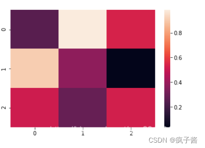 如下图
如下图
大家想要详细了解可以参考,其代码如下:
from matplotlib import pyplot as plt
import seaborn as sns
import numpy as np
import pandas as pd
from collections import Counter
from pandas.core.frame import DataFrame
zong = []
name = ['t1','t2','t3','t4']
# t1 t2 t3 t4  为不同时间窗口,大家可以根据自己情况进行调整
for names in name:
    fen = []
    a = pd.read_excel('e:/doc_topics__'+names+'.xlsx')
    # 这里我将每个时间窗口存储为一个xlsx,所以这里进行循环读取,并且将其主题归属存到xlsx里,方便
    # 下面进行强度计算。
    m = a['主题'].values.tolist()
    for i in range(len(m)):
        fen.append(m[i])
    zong.append(fen)

ht = []
for i in range(len(zong)):
    f = Counter(zong[i])
    print(f)
    dict_1 = dict(f)
    dictlist = []
    m = []
    for keys, value in dict_1.items():
        temp = (keys, value)
        dictlist.append(temp)
    a = len(zong[i])
    for j in range(len(dictlist)):
        s_t = dictlist[j][1]
        s_w = a
        HT = s_t/s_w
        m.append(HT)
    ht.append(m)
m1 = DataFrame(ht)
df2 = pd.DataFrame(m1.values.T, index=m1.columns, columns=m1.index)
df2.to_excel('e:/qiangdu1.xlsx')
# 最终将每个主题强度计算结果存入xlsx中
print(df2)
data=pd.read_excel('e:/qiangdu.xlsx')
print(data)
data.columns = ['0', '0', '0', '0']
data.index = ['topic0', 'topic1', 'topic2','topic3','topic4']
# 这我是因为我的主题数量只有五个 ,大家可以根据自己情况进行判断
# 下面是我用sns 进行的强度计算。
plot=sns.heatmap(data,cmap='YlGnBu',annot_kws={"fontsize":20})
plt.rcParams['font.sans-serif']=['SimHei']
plt.yticks(rotation = 360)
plt.show()
第四步:主题相似度,
这里是用的是主题词的权重,在这里我说明一下
列子:
这里有两个通过产生的主题t1与t2,如下:
t0 :('a',0.25),('b',0.23) ('c',0.23)
t1 :('b',0.25),('g',0.16) ,('a',0.11)
在我们进行相似度计算时需要将t0 与t1 中主题词一样的,进行位置互换,如下:
t0 : ('a',0.25),('b',0.23), ('c',0.23)
t1 : ('a',0.11),('b',0.25),('g',0.16)
这是通过主题词的权重即概率产生一个主题向量,即:
t0 = (0.25,0.23,0.23)
t1= (0.11,0.25,0.16)
这是我在用余弦值进行相似度计算即可,代码如下:
import numpy as np
from scipy.spatial.distance import pdist
from numpy import *

import numpy as np
def cosine_distance(vec1,vec2):
    Vec = np.vstack([vec1,vec2])
    dist2 = 1 - pdist(Vec, 'cosine')
    return dist2
# 余弦值计算方法
def lda_cos(list1,list2):
    a = []
    b = []
    for i in range(len(list1)):
        for j  in  range(len(list2)):
            if list1[i][0] == list2[j][0]:
                a.append(j)
                b.append(i)
                print(list1[i][0])
                print(list2[j][0])
    for i in range(len(a)):
        list2[a[i]],list2[b[i]] =  list2[b[i]] ,list2[a[i]]
    cos_dic1 = []
    cos_dic2 = []
    for i  in range(len(list1)):
        cos_dic1.append(list1[i][1])
        cos_dic2.append(list2[i][1])

    m =1-cosine_distance(cos_dic1, cos_dic2)
    return m
# 向量余弦值就算,在方法中已经将向量的互换方法写明,大家只需要将向量穿进去即可
# 源数据如下:  list1 = ('a',0.11),('b',0.25),('g',0.16)
def tumple_1(list1,list2):
    tuple_1 = []
    for  i  in range(len(list1)):
        a = [list1[i],list2[i]]
        tup_t = tuple(a)
        tuple_1.append(tup_t)
    return tuple_1

all = []
for i  in range(t1,t2,10):
    m = str(i)
    data = []
    sta  = []
    k = []
    with open('lda— ',encoding='utf8') as f: # 这里为之前的lda生成的存入txt的主题向量
        for line in f.readlines():
            line = line.strip("\n")
            line = line.split(",")
            data.append(line)
    for i in range(0,len(data),2):

        m = tumple_1(data[i], data[i+1])
        sta.append(m)
    k.append(sta)
    all.append(k)
print(len(all))
sim_all  = []
for m in range(len(all)-1):
    sim_lda35 = []
    for i in range(len(all[m][0])):
        ad = []
        for j in range(len(all[m+1][0])):
            la = lda_cos(all[m][0][i], all[m+1][0][j])
            ad.append(la[0])
        sim_lda35.append(ad)
    sim_all.append(sim_lda35)
print(sim_all)
print('--------------------')
m1 = []
for i in range(len(sim_all)):
    m2 = []
    for j in range(len(sim_all[i])):
        m3 = []
        a = sum(sim_all[i][j])
        for k in range(len(sim_all[i][j])):
            m = sim_all[i][j][k] / a
            m3.append(m)
        m2.append(m3)
    m1.append(m2)
for i in range(len(m1)):
    for j  in  range(len(m1[i])):
        print(m1[i][j])
print('----------')
print(m1)
#  大家可以忽略计算过程 只看m1  m1为一个多维列表,每个维度为当前时间窗口与下个时间窗口 主题之间相似度
第五步:
大家根据相似度结果画桑吉图,我用的是pyecharts
这里大家可以看这篇文章,或者去pyecharts官网进行学习:
Document pyecharts 官网
Pyecharts一文速学-绘制桑基图详解+Python代码_fanstuck的博客-CSDN博客_.render_notebook()
import json

from pyecharts import options as opts
from pyecharts.charts import Sankey
import pyecharts
pyecharts.globals._WarningControl.ShowWarning=False
nodes = [
    {"name": "1"},
    {"name": "2"},
    {"name": "3"},
    {"name": "4"},
    {"name": "5"},
    {"name": "6"},
    {"name": "7"},
    {"name": "8"},
    {"name": "9"},
]
links = [
    {"source": "1", "target": "4", "value": 5},
    {"source": "1", "target": "5", "value": 3},
    {"source": "2", "target": "4", "value": 5},
    {"source": "2", "target": "5", "value": 3},
    {"source": "2", "target": "7", "value": 3},
    {"source": "3", "target": "4", "value": 3},
    {"source": "3", "target": "5", "value": 3},
    {"source": "3", "target": "7", "value": 3},
    {"source": "4", "target": "8", "value": 15},
    {"source": "4", "target": "9", "value": 30},
]
pic = (
    Sankey()
        .add(
        "受访者人数",  # 设置图例名称
        nodes,  # 传入节点数据
        links,  # 传入边和流量数据
        linestyle_opt=opts.LineStyleOpts(opacity=0.5, curve=0.5, color="source"),
        # 设置透明度、弯曲度、颜色,color可以是"source"或"target"
        label_opts=opts.LabelOpts(position="right"),  # 设置标签位置,position可以是"top"、"left"、"right"、"bottom"等
        node_width=20,  # 设置节点矩形的宽度
        node_gap=10,  # 设置节点矩形的距离
    )
        .set_global_opts(title_opts=opts.TitleOpts(title="选择工作的最主要原因"))  # 设置图表标题
)
pic.render('e:/sanji.html')
谢谢大家的关注,最近因为学业可能回复较慢,但是一定会回复。
文章出处登录后可见!