主题建模:BERTopic(实战篇)
BERTopic 是基于深度学习的一种主题建模方法。 年底,
提出了
Bidirectional Encoder Representations from Transformers (BERT)。BERT 是一种用于 NLP 的预训练策略,它成功地利用了句子的深层语义信息
。
1.加载数据
本次实验数据使用的是 fetch_20newsgroups 数据集。
from sklearn.datasets import fetch_20newsgroups
dataset = fetch_20newsgroups(subset='train', remove=('headers', 'footers', 'quotes'))['data']
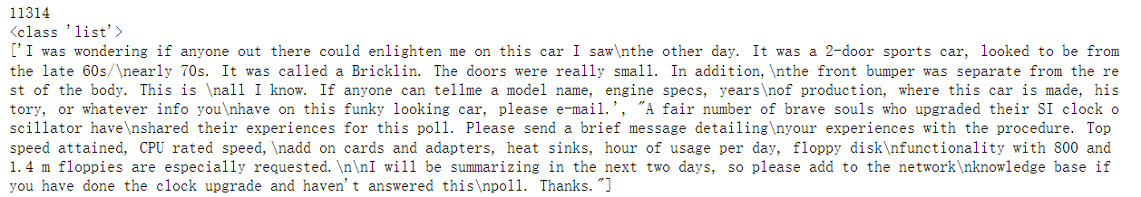
print(len(dataset)) # the length of the data
print(type(dataset)) # the type of variable the data is stored in
print(dataset[:2]) # the first instance of the content within the data
import pandas as pd
import numpy as np
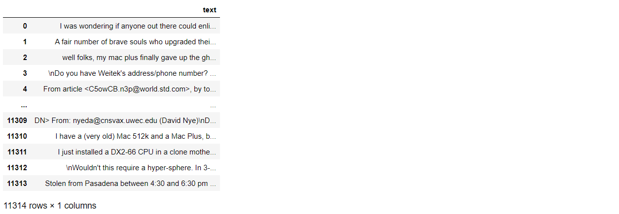
# Creating a dataframe from the data imported
full_train = pd.DataFrame()
full_train['text'] = dataset
full_train['text'] = full_train['text'].fillna('').astype(str) # removing any nan type objects
full_train
2.数据预处理
对于英文文本来说,一般是经过 分词、词形还原、去除停用词 等步骤,但也不是必须的。
import nltk
from nltk.stem import WordNetLemmatizer
from nltk.tokenize import word_tokenize
# If the following packages are not already downloaded, the following lines are needed
# nltk.download('wordnet')
# nltk.download('omw-1.4')
# nltk.download('punkt')

filtered_text = []

lemmatizer = WordNetLemmatizer()

for i in range(len(full_train)):
    text = lemmatizer.lemmatize(full_train.loc[i,'text'])
    text = text.replace('\n',' ')
    filtered_text.append(text)

filtered_text[:1]

3.BERTopic 建模
from bertopic import BERTopic
from sentence_transformers import SentenceTransformer
from umap import UMAP
from hdbscan import HDBSCAN
from bertopic.vectorizers import ClassTfidfTransformer

3.1 嵌入(Embeddings)
在 BERTopic 中,all-MiniLM-L6-v2 作为处理英文文本的默认嵌入模型,paraphrase-multilingual-MiniLM-L12-v2 提供对另外 多种语言的嵌入支持。当然,
Sentence-Transformers 还提供了很多其他的嵌入模型。
我们甚至可以不选择 Sentence-Transformers 提供的任何一种嵌入方法,而改用 Flair、Spacy、Gensim 等提供的嵌入方法,那么安装时候则需要选择:
pip install bertopic[flair]
pip install bertopic[gensim]
pip install bertopic[spacy]
注意:如果这些模型比较难下载,可以先从官网手动下载,再加载对应的路径即可。比如下面用到的 all-MiniLM-L6-v2 就是博主先手动下载到文件夹下的。
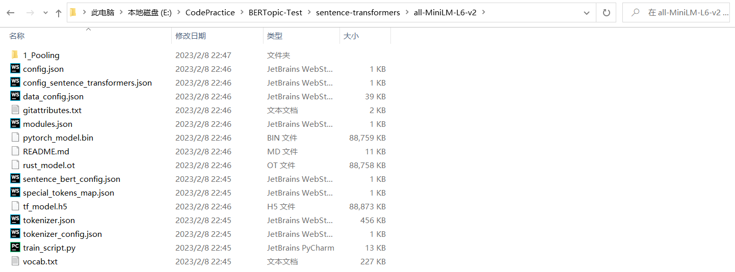
# Step 1 - Extract embeddings
embedding_model = SentenceTransformer('sentence-transformers/all-MiniLM-L6-v2')
3.2 降维(Dimensionality Reduction)
除了利用默认的 UMAP 降维,我们还可以使用 PCA、Truncated SVD、cuML UMAP 等降维技术。
# Step 2 - Reduce dimensionality
umap_model = UMAP(n_neighbors=15, n_components=5, min_dist=0.0, metric='cosine')
n_neighbors:此参数控制 UMAP 如何平衡数据中的局部结构与全局结构。值越小 UMAP 越专注于局部结构;值越大 UMAP 越专注于全局结构。n_components:该参数允许用户确定将嵌入数据的降维空间的维数。与其他一些可视化算法(例如t-SNE)不同,UMAP 在嵌入维度上具有很好的扩展性,不仅仅只能用于维或
维的可视化。
min_dist:该参数控制允许 UMAP 将点打包在一起的紧密程度。从字面上看,它提供了允许点在低维表示中的最小距离。值越小嵌入越密集。metric:该参数控制了如何在输入数据的环境空间中计算距离。
详情参见:https://umap-learn.readthedocs.io/en/latest/parameters.html
3.3 聚类(Clustering)
除了默认的 HDBSCAN,K-Means 聚类算法在原作者的实验上表现也非常好,当然也可以选择其他的聚类算法。
# Step 3 - Cluster reduced embeddings
hdbscan_model = HDBSCAN(min_cluster_size=15, metric='euclidean', cluster_selection_method='eom', prediction_data=True)
min_cluster_size:影响生成的聚类的主要参数。理想情况下,这是一个相对直观的参数来选择:将其设置为你希望考虑集群的最小大小的分组。cluster_selection_method:该参数确定 HDBSCAN 如何从簇树层次结构中选择平面簇。默认方法是eom,表示 Excess of Mass。prediction_data:确保 HDBSCAN 在拟合模型时进行一些额外的计算,从而显著加快以后的预测查询速度。
详情参见:https://hdbscan.readthedocs.io/en/latest/parameter_selection.html
3.4 序列化(Tokenizer)
from sklearn.feature_extraction.text import CountVectorizer
# Step 4 - Tokenize topics
vectorizer_model = CountVectorizer(stop_words="english")
3.5 加权(Weighting scheme)
此处的加权是利用了基于 TF-IDF 改进的 c-TF-IDF,也可以使用基于类 BM25 的加权方案,或者对 TF 进行开方处理。
- 基于类
BM25的加权方案: - 减少词频:
注:我在《文本相似度算法:TF-IDF与BM25》这篇博客中详细介绍了 BM25 算法。
# Step 5 - Create topic representation
ctfidf_model = ClassTfidfTransformer()
4.训练模型
topic_model = BERTopic(
    embedding_model=embedding_model,    # Step 1 - Extract embeddings
    umap_model=umap_model,              # Step 2 - Reduce dimensionality
    hdbscan_model=hdbscan_model,        # Step 3 - Cluster reduced embeddings
    vectorizer_model=vectorizer_model,  # Step 4 - Tokenize topics
    ctfidf_model=ctfidf_model,          # Step 5 - Extract topic words
    diversity=0.5,                      # Step 6 - Diversify topic words
    nr_topics=10
)
几个常用的参数:
diversity:是否使用MMR(Maximal Marginal Relevance,最大边际相关性)来多样化生成的主题表示。如果设置为None,则不会使用MMR。可接受的值介于和
之间,
nr_topics:指定主题数会将初始主题数减少到指定的值。这种减少可能需要一段时间,因为每次减少主题 () 都会激活
c-TF-IDF计算。如果将其设置为None,则不会应用任何减少。将其设置为‘auto’,则HDBSCAN自动减少主题。calculate_probabilities:默认为False。是否计算每篇文档所有主题的概率,而不是计算每篇文档指定主题的概率。如果文档较多(),这可能会减慢主题的提取速度。如果为
False,则不能使用相应的可视化方法visualize_probabilities。
博主测试的训练时间大概是 分钟。
topics, probabilities = topic_model.fit_transform(filtered_text)
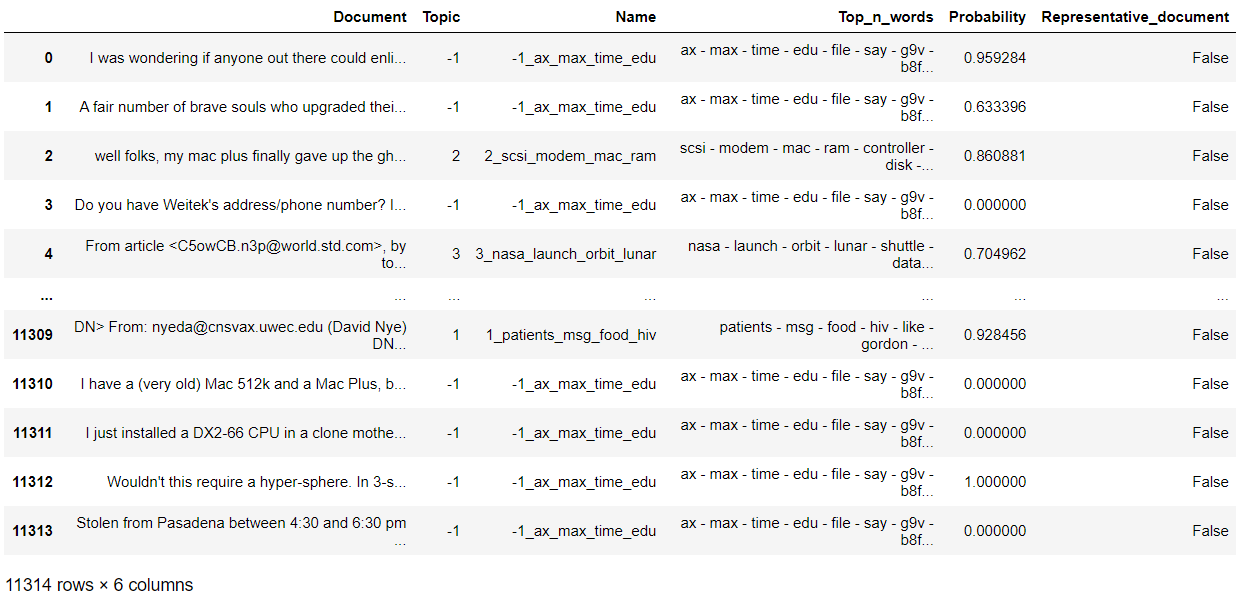
topic_model.get_document_info(filtered_text)
topic_model.get_topic_freq()

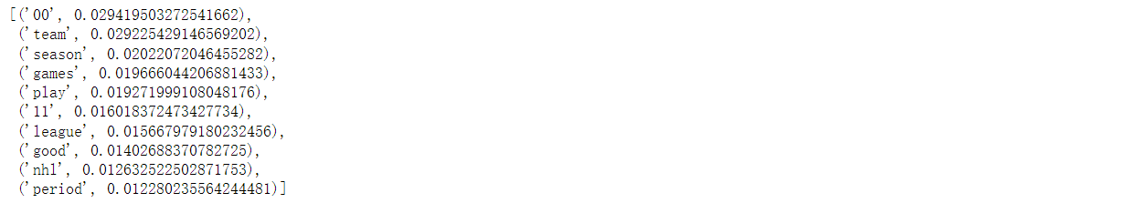
topic_model.get_topic(0)
5.可视化结果
BERTopic 提供了多种类型的可视化方法,以帮助我们从不同的方面评估模型。后续我会专门出一篇博客针对 BERTopic 中的可视化进行详细介绍,此处仅对一些常用的可视化方法进行总结。
5.1 Barchart
可视化所选主题的条形图。
topic_model.visualize_barchart()

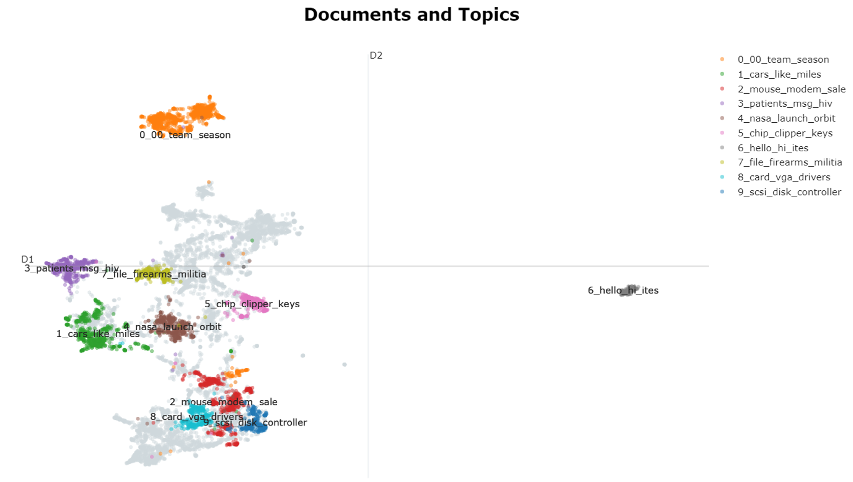
5.2 Documents
在 2D 中可视化文档及其主题。
embeddings = embedding_model.encode(filtered_text, show_progress_bar=False)

# Run the visualization with the original embeddings
topic_model.visualize_documents(filtered_text, embeddings=embeddings)
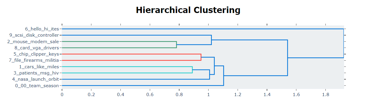
5.3 Hierarchy Topics
基于主题嵌入之间的余弦距离矩阵执行层次聚类。
topic_model.visualize_hierarchy()
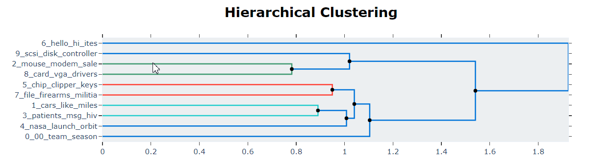
# Extract hierarchical topics and their representations
hierarchical_topics = topic_model.hierarchical_topics(filtered_text)

# Visualize these representations
topic_model.visualize_hierarchy(hierarchical_topics=hierarchical_topics)
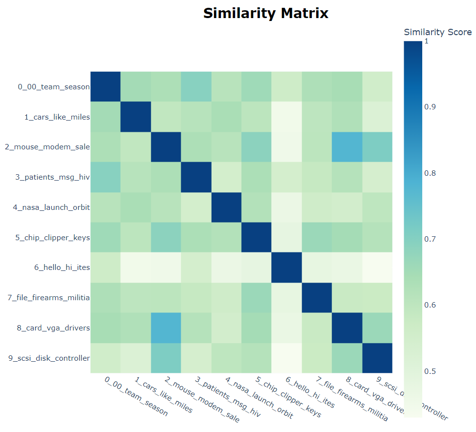
5.4 Heatmap
基于主题嵌入之间的余弦相似度矩阵,创建了一个热图来显示主题之间的相似度。
topic_model.visualize_heatmap()
5.5 Term Score Decline
每个主题都由一组单词表示。然而,这些词以不同的权重来代表主题。本可视化方法显示了需要多少单词来表示一个主题,以及随着单词的添加,增益在什么时候开始下降。
topic_model.visualize_term_rank()

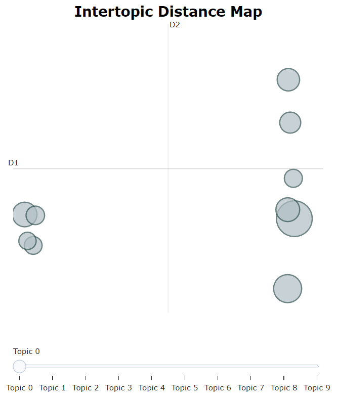
5.6 Topics
本可视化方法是受到了 LDAvis 的启发。LDAvis 是一种服务于 LDA 的可视化技术。
topic_model.visualize_topics()
6.评估
在 BERTopic 官网上并没有对评估这一块内容的介绍。但如果你想定量比较 LDA 和 BERTopic 的结果,则需要对评估方法加以掌握。
关于主题建模的评估方法,在我之前写的博客中也多次提到。可视化是一种良好的评估方法,但我们也希望以定量的方式对建模结果进行评估。主题连贯度(Topic Coherence)是最常用的评估指标之一。我们可以使用 Gensim 提供的 CoherenceModel 对结果进行进行评估。计算主题连贯度的方法很多,我们此处仅以 C_v 为例。
import gensim
import gensim.corpora as corpora
from gensim.models.coherencemodel import CoherenceModel
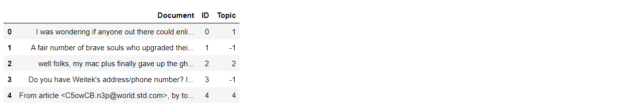
documents = pd.DataFrame({"Document": filtered_text,
                          "ID": range(len(filtered_text)),
                          "Topic": topics})
documents.head()
documents_per_topic = documents.groupby(['Topic'], as_index=False).agg({'Document': ' '.join})
documents_per_topic

cleaned_docs = topic_model._preprocess_text(documents_per_topic.Document.values)
# Extract vectorizer and analyzer from BERTopic
vectorizer = topic_model.vectorizer_model
analyzer = vectorizer.build_analyzer()
下面的内容主要涉及到 Gensim 中模型的使用,在我之前的博客中也有详细介绍,此处不再赘述。
# Extract features for Topic Coherence evaluation
words = vectorizer.get_feature_names()

tokens = [analyzer(doc) for doc in cleaned_docs]

dictionary = corpora.Dictionary(tokens)

corpus = [dictionary.doc2bow(token) for token in tokens]

topic_words = [[words for words, _ in topic_model.get_topic(topic)] for topic in range(len(set(topics))-1)]
不过,我们稍微看一下 topic_words 中的内容。
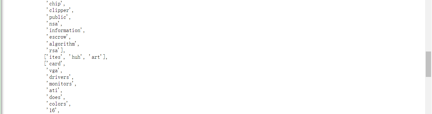
topic_words
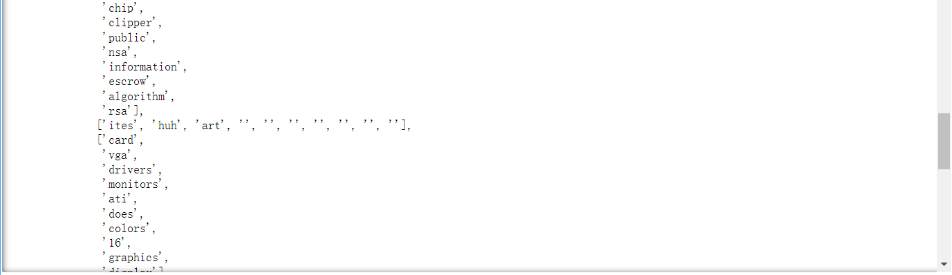
topic_words 的结果是一个双重列表,含义是每一个主题所对应的代表词组。从上图中可以看到,有一个列表的结果中包含空字符串,必须把这个空字符串去掉,不然后面的连贯度计算会报错。(注意:博主在这个地方一开始出现了错误,经排查才发现)
a = []
for i in range(len(topic_words)):
    b = []
    for word in topic_words[i]:
        if word != '':
            b.append(word)
    a.append(b)

topic_words = a
topic_words
# Evaluate
coherence_model = CoherenceModel(topics=topic_words,
                                 texts=tokens,
                                 corpus=corpus,
                                 dictionary=dictionary,
                                 coherence='c_v')

coherence = coherence_model.get_coherence()

print(coherence)

如果在一开始导入数据时,没有去除掉头尾的内容,按照下面这种方式导入,主题连贯度得分也会低不少。所以文本内容和有效的数据清理会对最后的结果会产生一定影响。
dataset = fetch_20newsgroups(subset='train')['data']

最后,对于本文中用到的几个包的版本特别说明一下。先安装 bertopic,再安装 gensim。
| 名称 | 版本 | 名称 | 版本 |
|---|---|---|---|
| pandas | 1.4.1 | numpy | 1.20.0 |
| bertopic | 0.13.0 | gensim | 3.8.3 |
| nltk | 3.8.1 | scikit-learn | 1.2.1 |
| scipy | 1.10.0 | sentence-transformers | 2.2.2 |
参考文献
-
[1] Devlin, J., Chang, M., Lee, K., & Toutanova, K. (2019). BERT: Pre-training of Deep Bidirectional Transformers for Language Understanding. ArXiv, abs/1810.04805.
-
[2] Soodeh Hosseini and Zahra Asghari Varzaneh. 2022. Deep text clustering using stacked AutoEncoder. Multimedia Tools Appl. 81, 8 (Mar 2022), 10861–10881. https://doi.org/10.1007/s11042-022-12155-0
文章出处登录后可见!