原文：Visit the VoxelMorph tutorial to learn about VoxelMorph and Learning-based Registration. Here’s an additional small tutorial on warping annotations together with images, and another on template (atlas) construction with VoxelMorph.

主要分为：

• Additional small tutorial 根据注释对图像进行变换
• VoxelMorph tutorial VoxelMorph教程
• Template (atlas) construction 模版搭建教程
  本文Github地址：https://github.com/MaybeRichard/VoxelMorph-explain

第一部分：Additional small tutorial 根据注释对图像进行变换

环境及背景介绍：

本部分的官方代码地址：https://colab.research.google.com/drive/1V0CutSIfmtgDJg1XIkEnGteJuw0u7qT-#scrollTo=h1KXYz-Nauwn
这一部分主要介绍的是如何使用vxm库里的方法对图像进行变换，代码中的方法是随机生成一个矩阵，然后根据该矩阵对图像进行仿射变换。
环境要求：tensorflow2.4,VoxelMorph
完整代码如下：

# 安装和导包
!pip install voxelmorph
import voxelmorph as vxm
import tensorflow as tf
import numpy as np
import matplotlib.pyplot as plt
 
# 对输入图像进行适当的预处理
pad_amt = 10
(x_train,_),_ = tf.keras.datasets.mnist.load_data()
# float64占用的内存是float32的两倍，是float16的4倍；比如对于CIFAR10数据集，如果采用float64来表示，需要60000323238/1024**3=1.4G，光把数据集调入内存就需要1.4G；如果采用float32，只需要0.7G，如果采用float16，只需要0.35G左右；占用内存的多少，会对系统运行效率有严重影响；（因此数据集文件都是采用uint8来存在数据，保持文件最小）
im = x_train[0,...].astype('float')/255
# np.pad(需要填充的array，((上，下),(左，右))，mode=constant...),这一步是为了增加边缘，累死padding，作用是防止后面的平移导致其超出范围
im = np.pad(im,((pad_amt,pad_amt),(pad_amt,pad_amt)))

# 手工创建变换矩阵
aff = np.eye(3) # 创建主对角矩阵
aff[:2,:2]+=np.random.randn(2,2)*0.1 # 在上半部分的2*2区域加入随机噪声
aff[:2, 2] = np.random.uniform(-10, 10, (2, )) # 均匀分布，(low,high,size) aff[:2, 2]的尺寸是(2,)
aff_inv = np.linalg.inv(aff)

margin=10
nb_annotations = 5
annotations = [np.random.uniform(margin,f-margin,nb_annotations) for f in im.shape] # 创建两个注释，(48,48)表示两个
annotations = np.stack(annotations,1)

# np.newaxis 的功能是增加新的维度，但是要注意 np.newaxis 放的位置不同，产生的矩阵形状也不同。放在第一个，给行上增加维度，放在最后一个，给列上增加维度
im_keras = im[np.newaxis,...,np.newaxis]
aff_keras = aff[np.newaxis,:2,:]
annotations_keras = annotations[np.newaxis,...]

# 进行仿射变换
im_warped = vxm.layers.SpatialTransformer()([im_keras, aff_keras])
im_warped = im_warped[0, ..., 0]

# get dense field of inverse affine
field_inv = vxm.utils.affine_to_dense_shift(aff_inv[:-1,:], im.shape, shift_center=True)[np.newaxis, ...]

# warp annotations
data = [tf.convert_to_tensor(f, dtype=tf.float32) for f in [annotations_keras, field_inv]]
annotations_warped = vxm.utils.point_spatial_transformer(data)[0, ...].numpy()

# 结果可视化
plt.figure()
# note that x and y need to be flipped due to xy indexing in matplotlib
plt.subplot(1, 2, 1)
plt.imshow(im, cmap='gray')
plt.plot(*[annotations[:, f] for f in [1, 0]], 'o')  
plt.axis('off')

plt.subplot(1, 2, 2)
plt.imshow(im_warped, cmap='gray')
plt.plot(*[annotations_warped[:, f] for f in [1, 0]], 'o')
plt.axis('off');

代码分析与讲解：

1. 库的导入：

!pip install voxelmorph
import voxelmorph as vxm
import tensorflow as tf
import numpy as np
import matplotlib.pyplot as plt

2. 图像的输入与预处理：

教程中使用的是mnist的数据集，数据集的预处理步骤包括:

• 对原始图像进行边缘填充
• 灰度归一化（具体作用参考：https://blog.csdn.net/qq_41383956/article/details/88593538）

# 加载mnist数据集
# 其标准输出应为： (x_train, y_train), (x_test, y_test)，但是只需要x_train数据展示，所以其他的丢掉
(x_train,_),_ = tf.keras.datasets.mnist.load_data()
# 灰度归一化，从0-255压缩到0-1
im = x_train[0,...].astype('float')/255
# 边缘填充
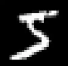
# 这一步的目的是，在后面对图像进行变换时，原本的Mnist数据集的28*28在变换后，
# 数字可能会移出图像区域，所以扩大原始数据的大小，也就是空白部分，方便展示变换的效果。
# pad_amt设置为10，及补充的区域为10个pixel
pad_amt = 10
# np.pad(需要填充的array，((上，下),(左，右))，mode=constant...),这一步是为了增加边缘，可以理解为padding
# 原始数据28*28，填补大小，上下左右各10，处理后数据48*48
im = np.pad(im,((pad_amt,pad_amt),(pad_amt,pad_amt)))

数据处理前后效果：

3. 手动创建变换矩阵：

# 手动生成仿射变换矩阵，方便后面affine操作

# 创建主对角矩阵
aff = np.eye(3) 
 # 在左上半部分的2*2区域加入随机噪声
aff[:2,:2]+=np.random.randn(2,2)*0.1
# 前两行的第三列的内容使用(-10,10)之间的均匀随机采样数字来替换
#  np.random.uniform(low,high,size)，使用(2,)的原因是aff[:2,2]数组就是一个两行一列的值
aff[:2, 2] = np.random.uniform(-10, 10, (2, ))
# 对上面计算后的矩阵求逆
aff_inv = np.linalg.inv(aff)

# 手动生成annotation变换矩阵，方便后面warp操作
margin=10
nb_annotations = 5
 # 创建一个列表，其中包含两个annotations，每个中包含nb_annotations个随机数字，范围在(margin,f-margin)之间
annotations = [np.random.uniform(margin,f-margin,nb_annotations) for f in im.shape]
# np.stack的简单用法在我的notion中有说明：
# https://sandy-property-d5e.notion.site/np-stack-48a69e31be084aa98cd15ce7d093c2ec
annotations = np.stack(annotations,1)

处理后的数据分别为：
aff_inv:

annotations:

4. Warp Data

# np.newaxis 的功能是增加新的维度。放在第一个，给行上增加维度，放在最后一个，给列上增加维度
im_keras = im[np.newaxis,...,np.newaxis] # (1, 48, 48, 1)
aff_keras = aff[np.newaxis,:2,:] #(1, 2, 3)
annotations_keras = annotations[np.newaxis,...] # (1,5,2)

# warp image
# 调用vxm库里的SpatialTransformer类，([im_keras, aff_keras])放在后面是什么用法暂时还没搞懂
# ([im_keras, aff_keras])分别代表的是图像数据和形变数据，通过空间变换将形变数据作用到图像数据中
im_warped = vxm.layers.SpatialTransformer()([im_keras, aff_keras])
im_warped = im_warped[0, ..., 0] # 取im_warped中的第0行第0列

# 获取取逆操作后的仿射矩阵的密集场Dense field
# 此处的affine_to_dense_shift和官方的教程不同，因为新版的vxm已经更新为此方法，此处已通过Issue询问过开发者
# vxm.utils.affine_to_dense_shift(array,shape,shift_center=True)
# 最后[np.newaxis, ...]的作用等价于field_inv = field_inv[np.newaxis, ...]，即给输出的结果的第一个位置增加一个维度
field_inv = vxm.utils.affine_to_dense_shift(aff_inv[:-1,:], im.shape, shift_center=True)[np.newaxis, ...]

# warp annotations
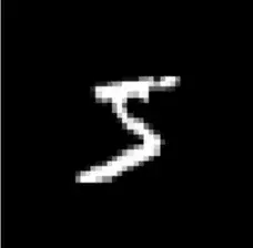
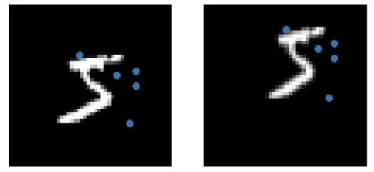
# 我的理解是：annotation是一些随机生成的点，在变换前后的图像中都是存在的
# 其作用是，帮助更明显的看出图像变化的方向和形式（涉及形变、整体移动的方向等信息）
# data为长度为2的列表，存储的分别是annotations_keras, field_inv，且两个都被转换为tf.Tensor形式，用于输入到vxm.utils.point_spatial_transformer中
data = [tf.convert_to_tensor(f, dtype=tf.float32) for f in [annotations_keras, field_inv]]
# 将辅助点和形变场都放入 vxm.utils.point_spatial_transformer，获取辅助点在该形变场下的变换信息
# [0,...]：从[1,5,2]中获取第0维度的信息=>[5,2]
annotations_warped = vxm.utils.point_spatial_transformer(data)[0, ...].numpy()

5.展示结果

plt.figure()
# 分别展示初始的图像和生成的辅助点
plt.subplot(1, 2, 1)
plt.imshow(im, cmap='gray')
plt.plot(*[annotations[:, f] for f in [1, 0]], 'o')  
plt.axis('off')

# 分别展示变换后的图像和变换后的辅助点
plt.subplot(1, 2, 2)
plt.imshow(im_warped, cmap='gray')
plt.plot(*[annotations_warped[:, f] for f in [1, 0]], 'o')
plt.axis('off');

第二部分：VoxelMorph tutorial VoxelMorph模型和训练教程

本部分的官方代码地址：https://colab.research.google.com/drive/1WiqyF7dCdnNBIANEY80Pxw_mVz4fyV-S?usp=sharing#scrollTo=joVczQLTPXMZ
这一部分主要介绍VoxelMorph基于深度学习的配准的实现，主要介绍以下四部分：

• MNIST数据集的介绍和使用
  如何处理数据集，建立模型，训练，配准和一般化的使用
• 现实的使用场景：颅脑MRI（2维切片）
  展示这些模型是如何在2d的颅脑数据上工作的，并展示更复杂场景下的使用
• 3D颅脑数据的使用
  展示完整3D图像的配准
• 高级功能
  使用更高级的功能，包括差分形态和微调模型

代码分析与讲解：

一、MNIST数据集的介绍和使用：

1.库的导入：

# 库的安装和导入
!pip install voxelmorph 
import os, sys
import numpy as np
import tensorflow as tf
assert tf.__version__.startswith('2.'), 'This tutorial assumes Tensorflow 2.0+'
import voxelmorph as vxm
import neurite as ne

2.数据的准备：

在这部分代码中，主要介绍2D MNIST数据的配准，在之后会尝试配准2维医学图像数据。如果数据量很小，可以将其加载到内存中，因为这样测试和训练起来更快。但是如果数据量很大的话，则需要按需扫描加载到内存中，这一点会在后续谈到。

# 导入MNIST数据集，需要使用到tensorflow.keras库
from tensorflow.keras.datasets import mnist
# 分别存储训练和测试数据
(x_train_load,y_train_load),(x_test_load,y_test_load) = mnist.load_data()
# 本文以数字5的图像配准为例
digit_sel = 5

# 分别获取下标为5的数据，分别存储为训练和测试集
x_train = x_train_load[y_train_load==digit_sel,...]
y_train = y_train_load[y_train_load==digit_sel]
x_test = x_test_load[y_test_load==digit_sel, ...]
y_test = y_test_load[y_test_load==digit_sel]

# 输出数据的尺寸以供检查
print('shape of x_train:{},y_train:{}'.format(x_train.shape,y_train.shape))

shape of x_train: (5421, 28, 28), y_train: (5421,)

测试/验证集的划分

ML的弯路：把数据只分在训练/测试中往往会导致问题的出现
反复（A）建立一个模型，（B）在训练数据上训练，（C）在测试数据上测试
这样做会导致过拟合（因为你会根据测试数据调整你的算法）。这在深度学习中是一个常见的错误。我们将把 “训练 “分成 “训练/验证 “数据，并把测试集留待以后使用。而只有在最后才会看测试数据。

# 抽出1000个作为验证集
nb_val = 1000
x_val = x_train[-nb_val:,...]
y_val = y_train[-nb_val:]
x_train = x_train[:-nb_val,...]
y_train = y_train[:-nb_val]

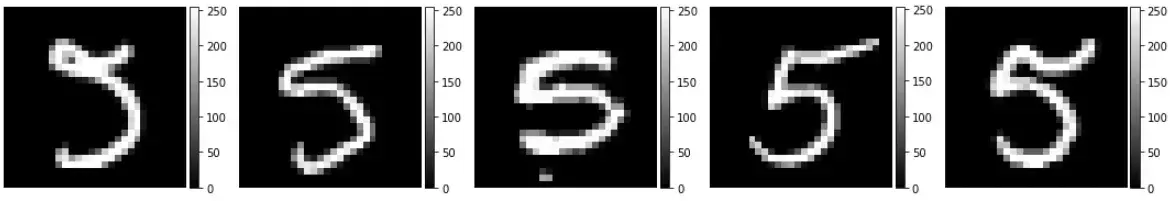
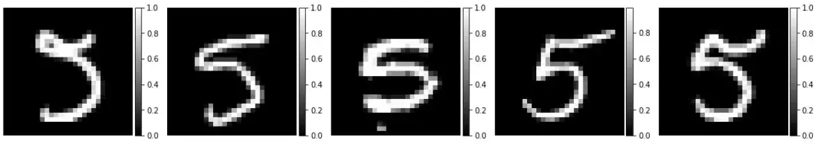
可视化数据

# numebr of visualize展示的数据的个数
nb_vis = 5
# nb.random.choice(需要抽取的数组，抽取的个数，是否允许重复)
idx = np.random.choice(x_train.shape[0],nb_vis,replace=False)
# example_digits是一个列表，存储的是分别是随机选择的数字的灰度值的矩阵
example_digits = [f for f in x_train[idx,...]]
# ne.plot.slices工具用来可视化数据
ne.plot.slices(example_digits,cmaps=['gray'],do_colorbars=True);

x_train = x_train.astype('float')/255
x_val = x_val.astype('float')/255
x_test = x_test.astype('float')/255

example_digits = [f for f in x_train[idx,...]]
ne.plot.slices(example_digits,camps=['gray'],do_colorbars=True];

扩展图像

# 从28*28拓展到32*32
# 第一维是图像个数，无需处理，后两维是长度和宽度
pad_amount = ((0,0),(2,2),(2,2))

x_train = np.pad(x_train,pad_amount,'constant')
x_val = np.pad(x_val,pad_amount,'constant')
x_text = np.pad(x_text,pad_amount,'constant')
print('shape of training data', x_train.shape)

shape of training data (4421, 32, 32)

3. CNN模型

提供参考和浮动图像，配准的目标是找到二者之间的变形矩阵。在基于学习的方法中，VoxelMorph选择两幅图像作为输入（参考和浮动图像，3232的MNIST数据），输出为密集形变场𝜙（3232*2，每个点表示像素的移动信息）。直观来说，密集形变场𝜙提供了两个图片之间的关系，并且告诉我们如何移动浮动图像使得其和参考图像尽可能的拟合。
注意： 配准也包括仿射变换，但是在这里选择忽略掉。
VoxelMorph库中提供了VxmDense模型类用来建立密集变形网络。在之后会介绍这个类，出于教学目的，将从头开始建立这个模型，以展示网络的各个组成部分。首先，抽象vxm.networks.Unet()模型。

# 配置unet输入形状（移动和固定图像的concat）
ndim = 2
unet_input_features = 2
#  输入尺寸，32*32*2，*x_train.shape[1:]表示对(5000,32,32)解包，获取32，32并与2拼接得到(32,32,2)
inshape = (*x_train.shape[1:],unet_input_features)

# 配置unet
nb_features = [
		[32,32,32,32],# encode层
		[32,32,32,32,32,16] # decoder层
]
# 建立模型，传入参数
unet = vxm.networks.Unet(inshape=inshape,nb_features=nb_features)

查看模型的输入和输出

print("input shape:",unet.input.shape)
print("output shape:",unet.output.shape)

input shape: (None, 32, 32, 2) output shape: (None, 32, 32, 16)
现在需要确保输出为2个features，代表每个voxel的变形情况

体素Voxel，可以理解为体积像素，是三维图像中点的表示方式。与之对应的像素Pixel，是二维图像中点的表示方式。参考：https://www.techtarget.com/whatis/definition/voxel

# 将结果变形成为一个流动场
# 将unet.output(None, 32, 32, 16)输入到二维卷积中，输入channel为2，kernel为3，padding方式为same
disp_tensor = tf.keras.layers.Conv2D(ndim,kernel_size=3,padding='same',name='disp')(unet.output)

# 查看输出形状
print("displacement shape",disp_tensor.shape)

# tf.keras.models.Model 将层分组到具有训练和推理功能的对象中
def_model = tf.keras.models.Model(unet.inputs,disp_tensor)

displacement tensor: (None, 32, 32, 2)
变形层现在可以和UNet模型共享权重，并在def_model中体现

4. 损失函数

目前已知形变场𝜙是网络的输出，现在需要设计合理的损失函数。
在有监督学习中，具有ground truth，𝜙𝑔𝑡，只需要计算MSE=‖𝜙−𝜙𝑔𝑡‖即可。

而在无监督学习的图像配准中，主要利用的经典配准方法中的损失函数。
在没有监督的情况下，如何知道当前的形变场是否是最优的呢？

1. 确保𝑚∘𝜙(图像m根据形变场𝜙进行扭转）后的结果接近于𝑓
2. 归一化𝜙（确保其足够平滑）

为了达到(1)中的结果，需要对浮动图像m进行扭转。也就是使用空间变换网络层spatial transformation network layer，本质上进行的是线性插值。关于空间变换网络的介绍：博客

# 建立空间变换层
spatial_transformer = vxm.layers.SpatialTransformer(name='transformer')
# 从unet输入的数据中提取第一帧
moving_image = tf.expand_dims(unet.input[...,0],axis=-1)
# 根据transformer来对浮动图像进行变形
moved_image_tensor = spatial_transformer([moving_image,disp_tensor])

为了确保浮动图像更接近参考图像，同时为了获取损失的平滑性（2），在输出中加入了二者的结合。

outputs = [moved_image_tensor,disp_tensor]
vxm_model = tf.keras.models.Model(inputs=unet.inouts,outputs=outputs)

上面所建立的模型，是VoxelMorph标准的dense结构网络，包括unet，位移场和最后的空间变换层。但是并不是每次搭建网络都需要这些步骤从头搭建，VoxelMorph库提供了更便捷的搭建方法，也就是VxmDense模型类，下面演示这种方法。

# 使用VxmDense建立网络模型
inshape = x_train.shape[1:]
vxm_model = vxm.networks.VxmDense(inshape,nb_features,int_steps=0)

int_steps=0是一个高级功能的选项，设置为0表示不开启，开启的话就为使用微分同胚功能，这一功能在后续会介绍到。
下面来看一下使用VxmDense生成模型的结构是否正确

print('input shape: ', ', '.join([str(t.shape) for t in vxm_model.inputs]))
print('output shape:', ', '.join([str(t.shape) for t in vxm_model.outputs]))

input shape: (None, 32, 32, 1), (None, 32, 32, 1)
output shape: (None, 32, 32, 1), (None, 32, 32, 2)

现在已经学会了如何快速的搭建网络。下面定义损失，在keras中，需要为每次的输出定义损失。第一个损失是简单的计算扭曲图像𝑚∘𝜙 的MSE。第二个损失函数，教程中选择位移的空间梯度作为损失。

# voxelmorph拥有内置的多个损失函数
losses = [vxm.losses.MSE().loss, vxm.losses.Grad('l2').loss]

# # 通常，会用超参数来平衡两种损失
lambda_param = 0.05
loss_weights = [1, lambda_param]

最后，开始编译模型，在模型的变异过程中，需要定义优化器和损失以及权重。

vxm_model.compile(optimizer='Adam', loss=losses, loss_weights=loss_weights)

5. 训练模型
为了训练，我们需要确保数据的格式是正确的，并且要满足keras的fed网络的要求。这也就需要数据在一个大的数组中或者是在model.fit_generator函数中，也就需要我们自定义python生成器。
下面定义一个简单的生成器作为演示，加载的是MINST数据。

def vxm_data_generator(x_data, batch_size=32):
    """
    生成器接收数据尺寸为[N,H,W]，输出数据传递给自定义的voxel模型。需要注意的是，每次的输入和输出需要提供的数据类型为numpy。
    
    inputs:  浮动图像 [bs, H, W, 1], 固定图像 [bs, H, W, 1]
    outputs: 移动后的浮动图像 [bs, H, W, 1], 0梯度模版 [bs, H, W, 2]
    """

    #初步确定尺寸
    vol_shape = x_data.shape[1:] # extract data shape
    ndims = len(vol_shape)
    
    # 准备一个为0的列表，尺寸和图像的输入尺寸相同
    zero_phi = np.zeros([batch_size, *vol_shape, ndims])
    
    while True:
        # 准备输入数据：
        # 图像的尺寸为： [batch_size, H, W, 1]
        # 分别随机参考和浮动图像的下标，随机数量为batchsize
        idx1 = np.random.randint(0, x_data.shape[0], size=batch_size)
        moving_images = x_data[idx1, ..., np.newaxis]
        idx2 = np.random.randint(0, x_data.shape[0], size=batch_size)
        fixed_images = x_data[idx2, ..., np.newaxis]
        inputs = [moving_images, fixed_images]
        
        # 准备输出(移动后的移动图像)
        # 当然，在当前步骤中是没有这个图像的，但是需要作为对比来计算损失（移动后的图像和固定图像之间的）
        # 此外，还希望给位移场增加惩罚项。
        outputs = [fixed_images, zero_phi]
        yield (inputs, outputs)

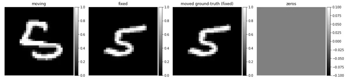
# 测试编写的生成器
train_generator = vxm_data_generator(x_train)
in_sample, out_sample = next(train_generator)

# 可视化
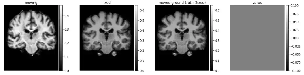
images = [img[0, :, :, 0] for img in in_sample + out_sample] 
titles = ['moving', 'fixed', 'moved ground-truth (fixed)', 'zeros']
ne.plot.slices(images, titles=titles, cmaps=['gray'], do_colorbars=True);

开始训练

nb_epochs = 10
steps_per_epoch = 100
hist = vxm_model.fit_generator(train_generator, epochs=nb_epochs, steps_per_epoch=steps_per_epoch, verbose=2);

Epoch 1/10
100/100 - 32s - loss: 0.0566 - transformer_loss: 0.0537 - flow_loss: 0.0572
Epoch 2/10
100/100 - 30s - loss: 0.0250 - transformer_loss: 0.0196 - flow_loss: 0.1092
Epoch 3/10
100/100 - 30s - loss: 0.0194 - transformer_loss: 0.0141 - flow_loss: 0.1053
Epoch 4/10
100/100 - 30s - loss: 0.0170 - transformer_loss: 0.0119 - flow_loss: 0.1021
Epoch 5/10
100/100 - 30s - loss: 0.0150 - transformer_loss: 0.0102 - flow_loss: 0.0963
Epoch 6/10
100/100 - 30s - loss: 0.0141 - transformer_loss: 0.0093 - flow_loss: 0.0950
Epoch 7/10
100/100 - 30s - loss: 0.0134 - transformer_loss: 0.0087 - flow_loss: 0.0929
Epoch 8/10
100/100 - 30s - loss: 0.0126 - transformer_loss: 0.0081 - flow_loss: 0.0901
Epoch 9/10
100/100 - 30s - loss: 0.0116 - transformer_loss: 0.0072 - flow_loss: 0.0877
Epoch 10/10
100/100 - 30s - loss: 0.0116 - transformer_loss: 0.0072 - flow_loss: 0.0870

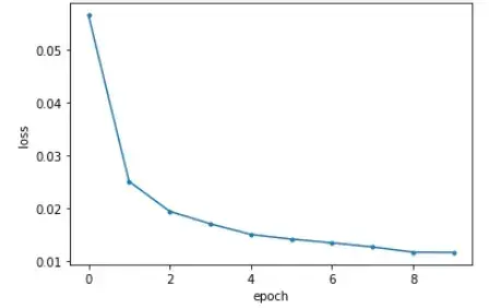
可视化损失函数曲线

import matplotlib.pyplot as plt

def plot_history(hist, loss_name='loss'):
    # Simple function to plot training history.
    plt.figure()
    plt.plot(hist.epoch, hist.history[loss_name], '.-')
    plt.ylabel('loss')
    plt.xlabel('epoch')
    plt.show()

plot_history(hist)

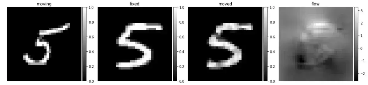
6. 配准

# 使用生成器加载验证集数据
val_generator = vxm_data_generator(x_val, batch_size = 1)
val_input, _ = next(val_generator)

# 使用predict函数实现配准
val_pred = vxm_model.predict(val_input)

# 输出计算时间
%timeit vxm_model.predict(val_input)

10 loops, best of 3: 41.9 ms per loop

可视化配准结果

# visualize
images = [img[0, :, :, 0] for img in val_input + val_pred] 
titles = ['moving', 'fixed', 'moved', 'flow']
ne.plot.slices(images, titles=titles, cmaps=['gray'], do_colorbars=True);

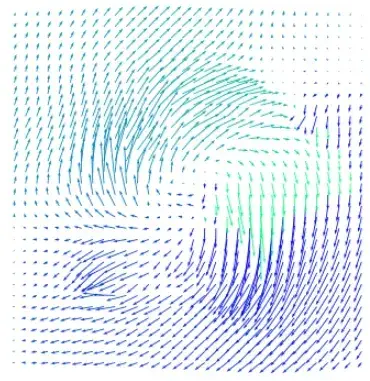
# 可视化密集场
ne.plot.flow([val_pred[1].squeeze()], width=5);

7. 一般化上述的方法和流程
使用训练好的模型预测数字7的配准结果，应该如何使用，效果如何？

# 提取数字7，归一化，补充为32*32
x_sevens = x_train_load[y_train_load==7, ...].astype('float') / 255
x_sevens = np.pad(x_sevens, pad_amount, 'constant')

# 配准预测
seven_generator = vxm_data_generator(x_sevens, batch_size=1)
seven_sample, _ = next(seven_generator)
seven_pred = vxm_model.predict(seven_sample)

# 可视化
images = [img[0, :, :, 0] for img in seven_sample + seven_pred] 
titles = ['moving', 'fixed', 'moved', 'flow']
ne.plot.slices(images, titles=titles, cmaps=['gray'], do_colorbars=True);

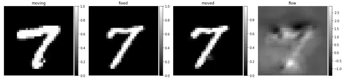
可以看到使用数字7也有不错的配准效果，究其原因是数字5存在部分的特征是和7相同的，也就是网络可以适配数字7的配准，但是对数字5的输入图像进行变形，增加一个权重，效果如何呢？

factor = 5
val_pred = vxm_model.predict([f * factor for f in val_input])

可视化
images = [img[0, :, :, 0] for img in val_input + val_pred] 
titles = ['moving', 'fixed', 'moved', 'flow']
ne.plot.slices(images, titles=titles, cmaps=['gray'], do_colorbars=True);

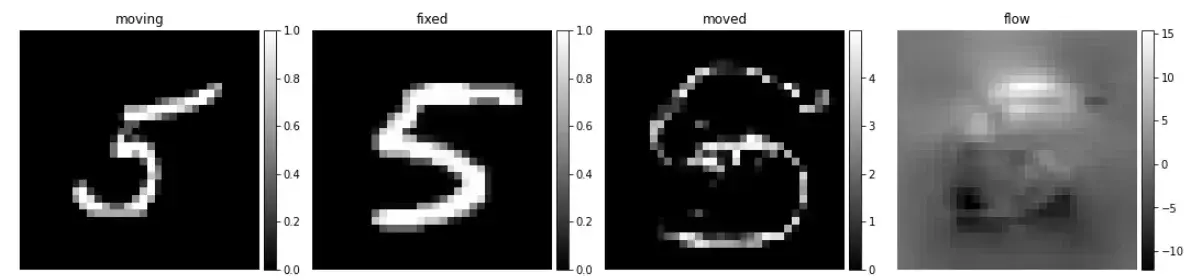
这样效果就会差很多，主要是因为网路从没见过这样的数据。

二、现实的使用场景：颅脑MRI（2维切片）

# 下载MRI数据集
!wget https://surfer.nmr.mgh.harvard.edu/pub/data/voxelmorph/tutorial_data.tar.gz -O data.tar.gz
!tar -xzvf data.tar.gz
# 加载并分类数据集
npz = np.load('tutorial_data.npz')
x_train = npz['train']
x_val = npz['validate']

# 208个体数据的尺寸为160*192
vol_shape = x_train.shape[1:]
print('train shape:', x_train.shape)

train shape: (208, 192, 160)

可视化部分数据

nb_vis = 5
idx = np.random.randint(0, x_train.shape[0], [5,])
example_digits = [f for f in x_train[idx, ...]]

# 可视化
ne.plot.slices(example_digits, cmaps=['gray'], do_colorbars=True);

2. 建立模型

vxm_model = vxm.networks.VxmDense(vol_shape, nb_features, int_steps=0)

# 定义损失和损失权重
losses = ['mse', vxm.losses.Grad('l2').loss]
loss_weights = [1, 0.01]

# 编译网络
vxm_model.compile(optimizer=tf.keras.optimizers.Adam(lr=1e-4), loss=losses, loss_weights=loss_weights)

# 幸运的是，这个数据和MNIST数据可以共用一个生成器，可以直接调用
train_generator = vxm_data_generator(x_train, batch_size=8)
in_sample, out_sample = next(train_generator)

# 可视化
images = [img[0, :, :, 0] for img in in_sample + out_sample]
titles = ['moving', 'fixed', 'moved ground-truth (fixed)', 'zeros']
ne.plot.slices(images, titles=titles, cmaps=['gray'], do_colorbars=True);

开始训练网络

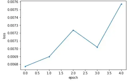
hist = vxm_model.fit_generator(train_generator, epochs=5, steps_per_epoch=5, verbose=2);

Epoch 1/5
5/5 - 13s - loss: 0.0068 - transformer_loss: 0.0068 - flow_loss: 9.9954e-08
Epoch 2/5
5/5 - 10s - loss: 0.0069 - transformer_loss: 0.0069 - flow_loss: 1.1938e-06
Epoch 3/5
5/5 - 10s - loss: 0.0072 - transformer_loss: 0.0072 - flow_loss: 6.1821e-06
Epoch 4/5
5/5 - 10s - loss: 0.0070 - transformer_loss: 0.0070 - flow_loss: 2.6120e-05
Epoch 5/5
5/5 - 10s - loss: 0.0076 - transformer_loss: 0.0076 - flow_loss: 7.4557e-05

画出训练曲线图

plot_history(hist)

出于时间成本，加载已经训练好200次的预训练模型。

vxm_model.load_weights('brain_2d_smooth.h5')
# 使用生成器加载验证集
val_generator = vxm_data_generator(x_val, batch_size = 1)
val_input, _ = next(val_generator)

# 预测
val_pred = vxm_model.predict(val_input)

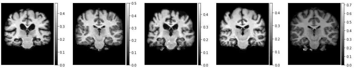
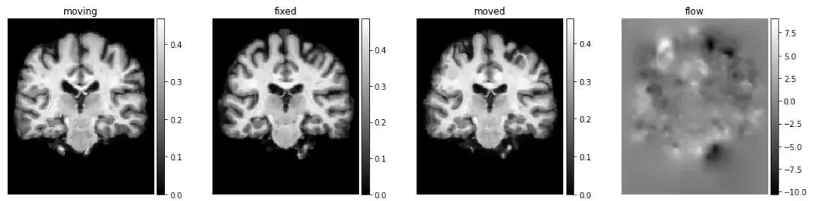
# 可视化
images = [img[0, :, :, 0] for img in val_input + val_pred] 
titles = ['moving', 'fixed', 'moved', 'flow']
ne.plot.slices(images, titles=titles, cmaps=['gray'], do_colorbars=True);

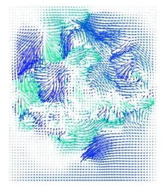
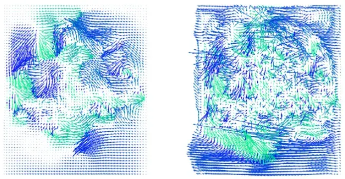
可视化变形场

flow = val_pred[1].squeeze()[::3,::3]
ne.plot.flow([flow], width=5);

3. 评价
分别对比使用MSE+smothness和MSE作为损失函数的网络学习效果。

# 使用 MSE + smoothness 损失
vxm_model.load_weights('brain_2d_smooth.h5')
our_val_pred = vxm_model.predict(val_input)

# 使用MSE损失
vxm_model.load_weights('brain_2d_no_smooth.h5')
mse_val_pred = vxm_model.predict(val_input)

# 分别可视化MSE+smothness和MSE的预测结果
images = [img[0, ..., 0] for img in [val_input[1], *our_val_pred]]
titles = ['fixed', 'MSE + smoothness', 'flow']
ne.plot.slices(images, titles=titles, cmaps=['gray'], do_colorbars=True);

images = [img[0, ..., 0] for img in [val_input[1], *mse_val_pred]]
titles = ['fixed', 'MSE only', 'flow']
ne.plot.slices(images, titles=titles, cmaps=['gray'], do_colorbars=True);

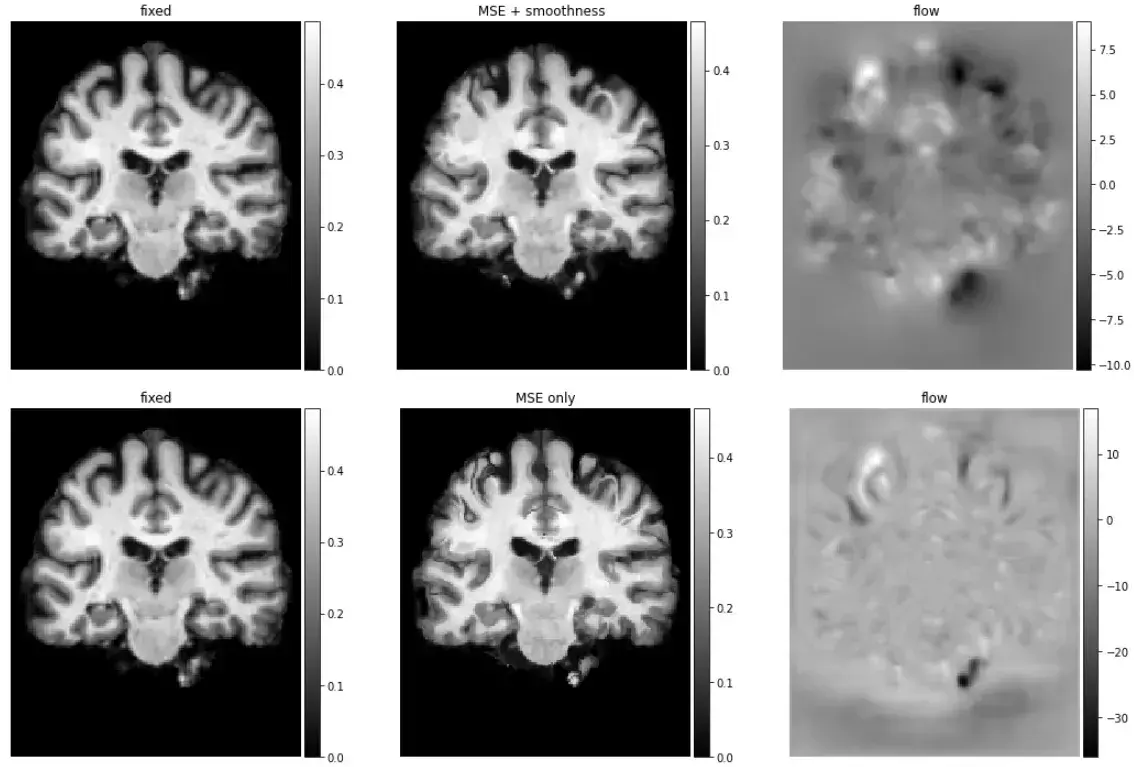
ne.plot.flow([img[1].squeeze()[::3, ::3] for img in [our_val_pred, mse_val_pred]], width=10);

三、3D颅脑数据的使用

最后，介绍一下3D数据下的模型建立。
由于模型和数据的大小，在教程的短暂实验中，无法展示模型的训练。作为替代，假设模型已经经过训练。可以自行尝试训练，步骤和2D数据基本相似。

1. 模型的建立

# 3D数据的尺寸为160,192,224
vol_shape = (160, 192, 224)
nb_features = [
    [16, 32, 32, 32],
    [32, 32, 32, 32, 32, 16, 16]
]
# build vxm network
vxm_model = vxm.networks.VxmDense(vol_shape, nb_features, int_steps=0);

2. 划分验证集

# 准备验证集
# seg数据集用于后面将分割数据作为辅助数据帮助网络训练的演示
val_volume_1 = np.load('subj1.npz')['vol']
seg_volume_1 = np.load('subj1.npz')['seg']
val_volume_2 = np.load('subj2.npz')['vol']
seg_volume_2 = np.load('subj2.npz')['seg']

val_input = [
	# 两个尺寸均为[1,160,192,224,1]
    val_volume_1[np.newaxis, ..., np.newaxis],
    val_volume_2[np.newaxis, ..., np.newaxis]
]

# 加载之前训练好的3D模型，因为数据太大，在教程中不演示训练过程
vxm_model.load_weights('brain_3d.h5')

# 开始配准
val_pred = vxm_model.predict(val_input);

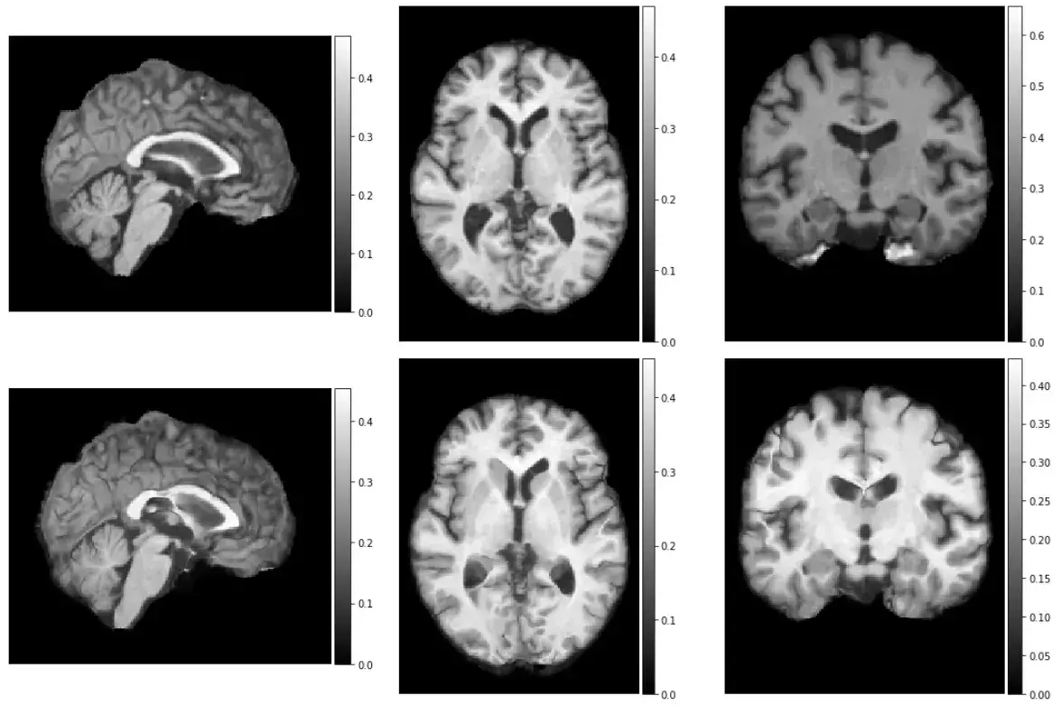
moved_pred = val_pred[0].squeeze()
pred_warp = val_pred[1]

mid_slices_fixed = [np.take(val_volume_2, vol_shape[d]//2, axis=d) for d in range(3)]
mid_slices_fixed[1] = np.rot90(mid_slices_fixed[1], 1)
mid_slices_fixed[2] = np.rot90(mid_slices_fixed[2], -1)

mid_slices_pred = [np.take(moved_pred, vol_shape[d]//2, axis=d) for d in range(3)]
mid_slices_pred[1] = np.rot90(mid_slices_pred[1], 1)
mid_slices_pred[2] = np.rot90(mid_slices_pred[2], -1)
ne.plot.slices(mid_slices_fixed + mid_slices_pred, cmaps=['gray'], do_colorbars=True, grid=[2,3]);

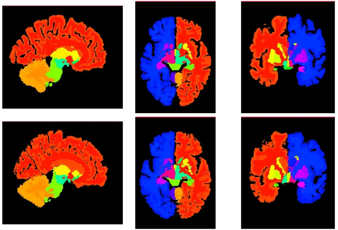
现在看一下分割数据的使用，在使用之前，需要对分割数据进行扭曲。

warp_model = vxm.networks.Transform(vol_shape,interp_method='nearest')
warped_seg = warp_model.predict([seg_volume_1[np.newaxis,...,np.newaxis], pred_warp])

下面需要准备一个色彩图

from pystrum.pytools.plot import jitter
import matplotlib

[ccmap, scrambled_cmap] = jitter(255, nargout=2)
scrambled_cmap[0, :] = np.array([0, 0, 0, 1])
ccmap = matplotlib.colors.ListedColormap(scrambled_cmap)

可视化分割的数据

mid_slices_fixed = [np.take(seg_volume_1, vol_shape[d]//1.8, axis=d) for d in range(3)]
mid_slices_fixed[1] = np.rot90(mid_slices_fixed[1], 1)
mid_slices_fixed[2] = np.rot90(mid_slices_fixed[2], -1)

mid_slices_pred = [np.take(warped_seg.squeeze(), vol_shape[d]//1.8, axis=d) for d in range(3)]
mid_slices_pred[1] = np.rot90(mid_slices_pred[1], 1)
mid_slices_pred[2] = np.rot90(mid_slices_pred[2], -1)

slices = mid_slices_fixed + mid_slices_pred
for si, slc  in enumerate(slices):
    slices[si][0] = 255
ne.plot.slices(slices, cmaps = [ccmap], grid=[2,3]);

查看运行时间

%timeit vxm_model.predict(val_input)

1 loop, best of 3: 37.1 s per loop
在测试中，一次完整的3D体数据运行需要10s，而对于传统方法则需要花费几个小时。