Pytorch: 全连接神经网络-解决 Boston 房价回归问题
Copyright: Jingmin Wei, Pattern Recognition and Intelligent System, School of Artificial and Intelligence, Huazhong University of Science and Technology
MLP 回归模型
使用sklearn库的fetch_california_housing()函数。数据集共包含20640个样本,有8个自变量。
import numpy as np
import pandas as pd
from sklearn.preprocessing import StandardScaler
from sklearn.model_selection import train_test_split
from sklearn.metrics import mean_squared_error, mean_absolute_error
from sklearn.datasets import fetch_california_housing

import torch
import torch.nn as nn
import torch.nn.functional as F
from torch.optim import SGD
import torch.utils.data as Data
import matplotlib.pyplot as plt
import seaborn as sns
房价数据准备
# 导入数据
housedata = fetch_california_housing()
# 切分训练集和测试集
X_train, X_test, y_train, y_test = train_test_split(housedata.data, housedata.target,
                                                    test_size = 0.3, random_state = 42)
70% 训练集,30%测试集。
X_train, X_test, y_train, y_test
(array([[   4.1312    ,   35.        ,    5.88235294, ...,    2.98529412,
           33.93      , -118.02      ],
        [   2.8631    ,   20.        ,    4.40120968, ...,    2.0141129 ,
           32.79      , -117.09      ],
        [   4.2026    ,   24.        ,    5.61754386, ...,    2.56491228,
           34.59      , -120.14      ],
        ...,
        [   2.9344    ,   36.        ,    3.98671727, ...,    3.33206831,
           34.03      , -118.38      ],
        [   5.7192    ,   15.        ,    6.39534884, ...,    3.17889088,
           37.58      , -121.96      ],
        [   2.5755    ,   52.        ,    3.40257649, ...,    2.10869565,
           37.77      , -122.42      ]]),
 array([[   1.6812    ,   25.        ,    4.19220056, ...,    3.87743733,
           36.06      , -119.01      ],
        [   2.5313    ,   30.        ,    5.03938356, ...,    2.67979452,
           35.14      , -119.46      ],
        [   3.4801    ,   52.        ,    3.97715472, ...,    1.36033229,
           37.8       , -122.44      ],
        ...,
        [   3.512     ,   16.        ,    3.76228733, ...,    2.36956522,
           33.67      , -117.91      ],
        [   3.65      ,   10.        ,    5.50209205, ...,    3.54751943,
           37.82      , -121.28      ],
        [   3.052     ,   17.        ,    3.35578145, ...,    2.61499365,
           34.15      , -118.24      ]]),
 array([1.938, 1.697, 2.598, ..., 2.221, 2.835, 3.25 ]),
 array([0.477  , 0.458  , 5.00001, ..., 2.184  , 1.194  , 2.098  ]))
# 数据标准化处理
scale = StandardScaler()
X_train_s = scale.fit_transform(X_train)
X_test_s = scale.transform(X_test)
# 将训练数据转为数据表
housedatadf = pd.DataFrame(data=X_train_s, columns = housedata.feature_names)
housedatadf['target'] = y_train
housedatadf
| MedInc | HouseAge | AveRooms | AveBedrms | Population | AveOccup | Latitude | Longitude | target | |
|---|---|---|---|---|---|---|---|---|---|
| 0 | 0.133506 | 0.509357 | 0.181060 | -0.273850 | -0.184117 | -0.010825 | -0.805682 | 0.780934 | 1.93800 |
| 1 | -0.532218 | -0.679873 | -0.422630 | -0.047868 | -0.376191 | -0.089316 | -1.339473 | 1.245270 | 1.69700 |
| 2 | 0.170990 | -0.362745 | 0.073128 | -0.242600 | -0.611240 | -0.044800 | -0.496645 | -0.277552 | 2.59800 |
| 3 | -0.402916 | -1.155565 | 0.175848 | -0.008560 | -0.987495 | -0.075230 | 1.690024 | -0.706938 | 1.36100 |
| 4 | -0.299285 | 1.857152 | -0.259598 | -0.070993 | 0.086015 | -0.066357 | 0.992350 | -1.430902 | 5.00001 |
| … | … | … | … | … | … | … | … | … | … |
| 14443 | 1.308827 | 0.509357 | 0.281603 | -0.383849 | -0.675265 | -0.007030 | -0.875918 | 0.810891 | 2.29200 |
| 14444 | -0.434100 | 0.350793 | 0.583037 | 0.383154 | 0.285105 | 0.063443 | -0.763541 | 1.075513 | 0.97800 |
| 14445 | -0.494787 | 0.588640 | -0.591570 | -0.040978 | 0.287736 | 0.017201 | -0.758858 | 0.601191 | 2.22100 |
| 14446 | 0.967171 | -1.076283 | 0.390149 | -0.067164 | 0.306154 | 0.004821 | 0.903385 | -1.186252 | 2.83500 |
| 14447 | -0.683202 | 1.857152 | -0.829656 | -0.087729 | 1.044630 | -0.081672 | 0.992350 | -1.415923 | 3.25000 |
14448 rows × 9 columns
使用相关系数热力图分析数据集中9个变量的相关性
datacor = np.corrcoef(housedatadf.values, rowvar=0)
datacor = pd.DataFrame(data = datacor, columns = housedatadf.columns,
                       index = housedatadf.columns)
plt.figure(figsize=(8, 6))
ax = sns.heatmap(datacor, square = True, annot = True, fmt = '.3f',
                 linewidths = .5, cmap = 'YlGnBu',
                 cbar_kws = {'fraction': 0.046, 'pad': 0.03})
plt.show()
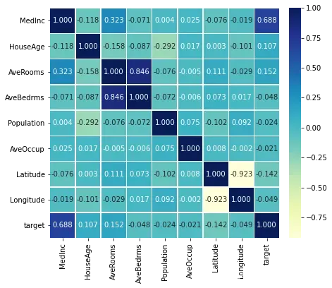
从图像可以看出,和目标函数相关性最大的是MedInc(收入中位数)变量。而且AveRooms和AveBedrms两个变量的正相关性较强。
# 将数据集转为张量
X_train_t = torch.from_numpy(X_train_s.astype(np.float32))
y_train_t = torch.from_numpy(y_train.astype(np.float32))
X_test_t = torch.from_numpy(X_test_s.astype(np.float32))
y_test_t = torch.from_numpy(y_test.astype(np.float32))
# 将训练数据处理为数据加载器
train_data = Data.TensorDataset(X_train_t, y_train_t)
test_data = Data.TensorDataset(X_test_t, y_test_t)
train_loader = Data.DataLoader(dataset = train_data, batch_size = 64,
                               shuffle = True, num_workers = 1)
搭建网络预测房价
# 搭建全连接神经网络回归
class MLPregression(nn.Module):
    def __init__(self):
        super(MLPregression, self).__init__()
        # 第一个隐含层
        self.hidden1 = nn.Linear(in_features=8, out_features=100, bias=True)
        # 第二个隐含层
        self.hidden2 = nn.Linear(100, 100)
        # 第三个隐含层
        self.hidden3 = nn.Linear(100, 50)
        # 回归预测层
        self.predict = nn.Linear(50, 1)

    # 定义网络前向传播路径
    def forward(self, x):
        x = F.relu(self.hidden1(x))
        x = F.relu(self.hidden2(x))
        x = F.relu(self.hidden3(x))
        output = self.predict(x)
        # 输出一个一维向量
        return output[:, 0]
# 输出网络结构
from torchsummary import summary
testnet = MLPregression()
summary(testnet, input_size=(1, 8)) # 表示1个样本,每个样本有8个特征
----------------------------------------------------------------
        Layer (type)               Output Shape         Param #
================================================================
            Linear-1               [-1, 1, 100]             900
            Linear-2               [-1, 1, 100]          10,100
            Linear-3                [-1, 1, 50]           5,050
            Linear-4                 [-1, 1, 1]              51
================================================================
Total params: 16,101
Trainable params: 16,101
Non-trainable params: 0
----------------------------------------------------------------
Input size (MB): 0.00
Forward/backward pass size (MB): 0.00
Params size (MB): 0.06
Estimated Total Size (MB): 0.06
----------------------------------------------------------------
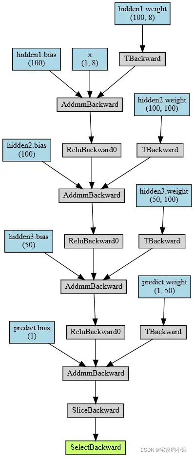
# 输出网络结构
from torchviz import make_dot
testnet = MLPregression()
x = torch.randn(1, 8).requires_grad_(True)
y = testnet(x)
myMLP_vis = make_dot(y, params=dict(list(testnet.named_parameters()) + [('x', x)]))
myMLP_vis
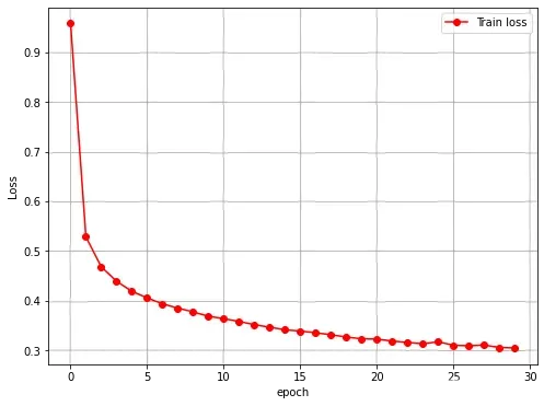
然后使用训练集对网络进行训练
# 定义优化器
optimizer = torch.optim.SGD(testnet.parameters(), lr = 0.01)
loss_func = nn.MSELoss() # 均方根误差损失函数
train_loss_all = []

# 对模型迭代训练,总共epoch轮
for epoch in range(30):
    train_loss = 0
    train_num = 0
    # 对训练数据的加载器进行迭代计算
    for step, (b_x, b_y) in enumerate(train_loader):
        output = testnet(b_x) # MLP在训练batch上的输出
        loss = loss_func(output, b_y) # 均方根损失函数
        optimizer.zero_grad() # 每次迭代梯度初始化0
        loss.backward() # 反向传播,计算梯度
        optimizer.step() # 使用梯度进行优化
        train_loss += loss.item() * b_x.size(0)
        train_num += b_x.size(0)
    train_loss_all.append(train_loss / train_num)
# 可视化损失函数的变换情况
plt.figure(figsize = (8, 6))
plt.plot(train_loss_all, 'ro-', label = 'Train loss')
plt.legend()
plt.grid()
plt.xlabel('epoch')
plt.ylabel('Loss')
plt.show()
对网络预测,并使用平均绝对值误差来表示预测效果
y_pre = testnet(X_test_t)
y_pre = y_pre.data.numpy()
mae = mean_absolute_error(y_test, y_pre)
print('在测试集上的绝对值误差为:', mae)
在测试集上的绝对值误差为: 0.39334159455403034
真实集和预测值可视化,查看之间的差异
index = np.argsort(y_test)
plt.figure(figsize=(8, 6))
plt.plot(np.arange(len(y_test)), y_test[index], 'r', label = 'Original Y')
plt.scatter(np.arange(len(y_pre)), y_pre[index], s = 3, c = 'b', label = 'Prediction')
plt.legend(loc = 'upper left')
plt.grid()
plt.xlabel('Index')
plt.ylabel('Y')
plt.show()
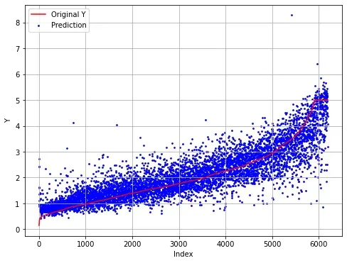
在测试集上,MLP回归正确地预测处理原始数据的变化趋势,但部分样本的预测差异较大。
文章出处登录后可见!
已经登录?立即刷新