如有错误,恳请指出。
文章目录
- 1. 在图像上绘制2d、3d标注框
- 2. 在图像上绘制Lidar投影
- 3. Lidar绘制前视图(FOV)
- 4. Lidar绘制前视图(FOV)+3d box
- 5. Lidar绘制鸟瞰图(BEV)
- 6. Lidar绘制鸟瞰图(BEV)+2d box
- 7. Lidar绘制全景图(RV)
- 8. Lidar绘制全景图(RV)+2d box
在对KITTI数据集的点云处理流程中,涉及鸟瞰图,前视图,全景图等多种视角。这篇笔记就是用来记录如何对点云进行多种视图的切换,以及如何实现在多种视图中进行标注框的展现。涵盖标注框的鸟瞰图的显示、在前视图中的显示以及在全景图中的显示。
这里主要是对代码的解析与思路的介绍,对于kitti数据集各种可视化展示可以查看之前写的另外一篇博客:KITTI数据集可视化(一):点云多种视图的可视化实现
1. 在图像上绘制2d、3d标注框
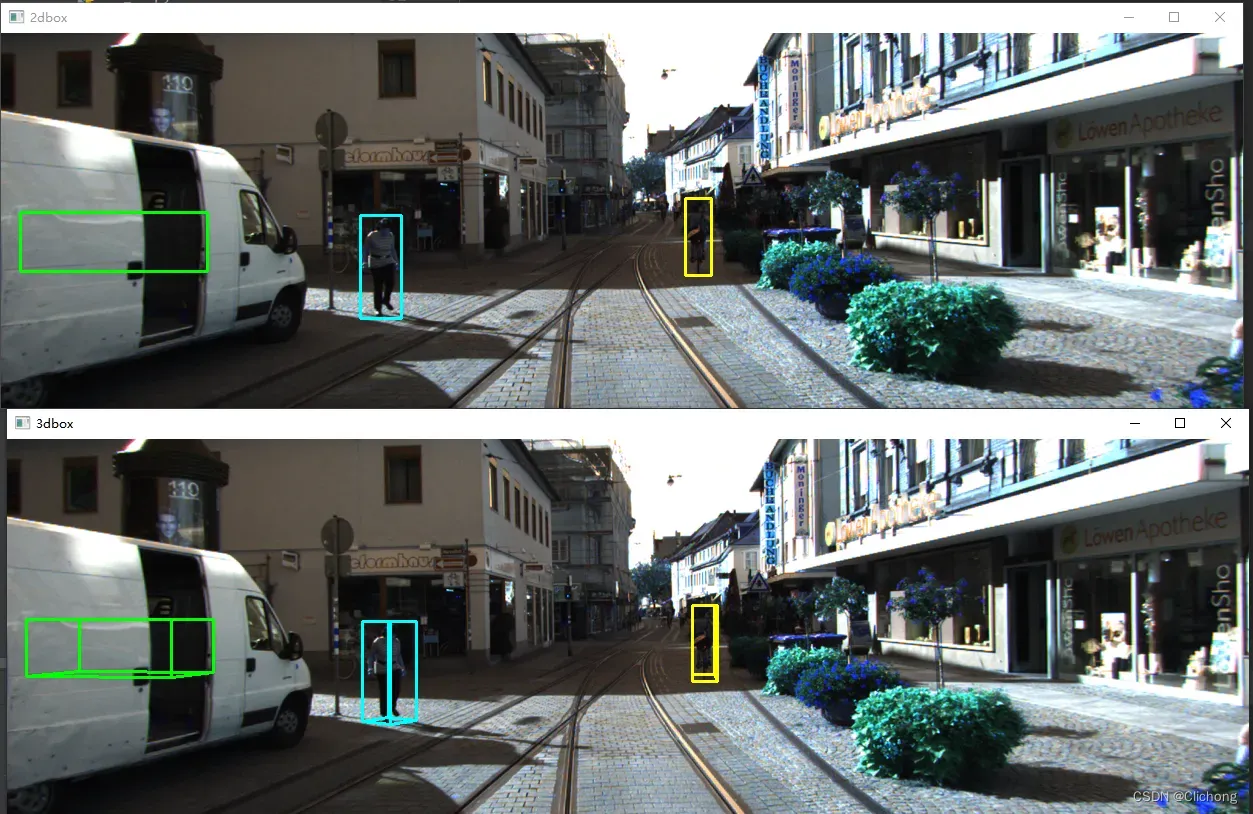
2d:对于2d标注框,在label中的第5~8列(浮点数)既是物体的2D边界框大小(bbox)。对这个2d边界框可以直接利用画框函数显示在原图像中。
3d:而对于3d标注框,首先在原点按照对象尺寸构建坐标点,然后利用ry旋转角度对目标进行旋转随后再平移到标注尺寸中。
def show_image_with_3d_boxes(self):
    show_image_with_boxes(self.img, self.objects, self.calib, show3d=True)
    cv2.waitKey(0)

def show_image_with_boxes(img, objects, calib, show3d=True, depth=None):
    """ Show image with 2D bounding boxes """
    img1 = np.copy(img)  # for 2d bbox
    img2 = np.copy(img)  # for 3d bbox
    #img3 = np.copy(img)  # for 3d bbox
    #TODO: change the color of boxes
    for obj in objects:
        if obj.type == "DontCare":
            continue
        if obj.type == "Car":
            cv2.rectangle(
            img1,
            (int(obj.xmin), int(obj.ymin)),
            (int(obj.xmax), int(obj.ymax)),
            (0, 255, 0),
            2,
        )
        if obj.type == "Pedestrian":
            cv2.rectangle(
            img1,
            (int(obj.xmin), int(obj.ymin)),
            (int(obj.xmax), int(obj.ymax)),
            (255, 255, 0),
            2,
        )
        if obj.type == "Cyclist":
            cv2.rectangle(
            img1,
            (int(obj.xmin), int(obj.ymin)),
            (int(obj.xmax), int(obj.ymax)),
            (0, 255, 255),
            2,
        )
        box3d_pts_2d, _ = utils.compute_box_3d(obj, calib.P)    # 获得3d框在图像上的投影(8个点,8x2)
        if box3d_pts_2d is None:
            print("something wrong in the 3D box.")
            continue

        # 绘制图像上的3d框投影
        if obj.type == "Car":
            img2 = utils.draw_projected_box3d(img2, box3d_pts_2d, color=(0, 255, 0))
        elif obj.type == "Pedestrian":
            img2 = utils.draw_projected_box3d(img2, box3d_pts_2d, color=(255, 255, 0))
        elif obj.type == "Cyclist":
            img2 = utils.draw_projected_box3d(img2, box3d_pts_2d, color=(0, 255, 255))

        # project
        # box3d_pts_3d_velo = calib.project_rect_to_velo(box3d_pts_3d)
        # box3d_pts_32d = utils.box3d_to_rgb_box00(box3d_pts_3d_velo)
        # box3d_pts_32d = calib.project_velo_to_image(box3d_pts_3d_velo)
        # img3 = utils.draw_projected_box3d(img3, box3d_pts_32d)
    # print("img1:", img1.shape)

    cv2.imshow("2dbox", img1)
    # print("img3:",img3.shape)
    # Image.fromarray(img3).show()
    show3d = True
    if show3d:
        # print("img2:",img2.shape)
        cv2.imshow("3dbox", img2)
    if depth is not None:
        cv2.imshow("depth", depth)

    return img1, img2

def compute_box_3d(obj, P):
    """ Takes an object and a projection matrix (P) and projects the 3d
        bounding box into the image plane.
        Returns:
            corners_2d: (8,2) array in left image coord.
            corners_3d: (8,3) array in rect camera coord.
    """
    # compute rotational matrix around yaw axis
    R = roty(obj.ry)

    # 3d bounding box dimensions
    l = obj.l
    w = obj.w
    h = obj.h

    # 3d bounding box corners:
    # 坐标系: 前x-右z-上y
    # qs: (8,3) array of vertices for the 3d box in following order:
    #             1 -------- 0
    #            /|         /|
    #           2 -------- 3 .
    #           | |        | |
    #           . 5 -------- 4
    #           |/         |/
    #           6 -------- 7
    x_corners = [l / 2, l / 2, -l / 2, -l / 2, l / 2, l / 2, -l / 2, -l / 2]
    y_corners = [0, 0, 0, 0, -h, -h, -h, -h]
    z_corners = [w / 2, -w / 2, -w / 2, w / 2, w / 2, -w / 2, -w / 2, w / 2]

    # rotate and translate 3d bounding box
    corners_3d = np.dot(R, np.vstack([x_corners, y_corners, z_corners]))

    # print corners_3d.shape: location (x,y,z) in camera coord
    corners_3d[0, :] = corners_3d[0, :] + obj.t[0]
    corners_3d[1, :] = corners_3d[1, :] + obj.t[1]
    corners_3d[2, :] = corners_3d[2, :] + obj.t[2]
    # print 'cornsers_3d: ', corners_3d
    # only draw 3d bounding box for objs in front of the camera
    if np.any(corners_3d[2, :] < 0.1):
        corners_2d = None
        return corners_2d, np.transpose(corners_3d)

    # project the 3d bounding box into the image plane
    # 投影到图像的具体实现是与内参矩阵P作用, 然后进行归一化,如果需要将点云坐标投影到像平面还需要除以Z,
    # 提取前两列数据既分别是xy轴数据
    corners_2d = project_to_image(np.transpose(corners_3d), P)    # 此时相当于在修正后的相机坐标系下
    # print 'corners_2d: ', corners_2d
    return corners_2d, np.transpose(corners_3d)

def project_to_image(pts_3d, P):
    """ Project 3d points to image plane.

    Usage: pts_2d = projectToImage(pts_3d, P)
      input: pts_3d: nx3 matrix
             P:      3x4 projection matrix
      output: pts_2d: nx2 matrix

      P(3x4) dot pts_3d_extended(4xn) = projected_pts_2d(3xn)
      => normalize projected_pts_2d(2xn)

      <=> pts_3d_extended(nx4) dot P'(4x3) = projected_pts_2d(nx3)
          => normalize projected_pts_2d(nx2)
    """
    n = pts_3d.shape[0]
    pts_3d_extend = np.hstack((pts_3d, np.ones((n, 1))))
    # print(('pts_3d_extend shape: ', pts_3d_extend.shape))
    pts_2d = np.dot(pts_3d_extend, np.transpose(P))  # nx3
    pts_2d[:, 0] /= pts_2d[:, 2]
    pts_2d[:, 1] /= pts_2d[:, 2]
    return pts_2d[:, 0:2]
2. 在图像上绘制Lidar投影
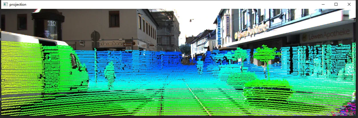
对于点云需要进行外参矩阵、R0校准矩阵、内参矩阵的转化后,才投影到相机图像的坐标系中。为了体现每个点的深度,可以使用R0校准后的矩阵,此时即为z轴信息可以体现在图像上的深度信息,这个信息可以来进行颜色深度图的控制
def show_lidar_on_image(pc_velo, img, calib, img_width, img_height):
    """ Project LiDAR points to image """
    img = np.copy(img)
    # 返回筛选后的原始点、筛选前的图像投影点、筛选的判断布尔结果
    imgfov_pc_velo, pts_2d, fov_inds = get_lidar_in_image_fov(
        pc_velo, calib, 0, 0, img_width, img_height, True
    )
    imgfov_pts_2d = pts_2d[fov_inds, :]     # 筛选后的投影点,已转化到图像坐标系上
    imgfov_pc_rect = calib.project_velo_to_rect(imgfov_pc_velo)    # 得到相机坐标系下的坐标,包含深度信息

    import matplotlib.pyplot as plt

    cmap = plt.cm.get_cmap("hsv", 256)
    cmap = np.array([cmap(i) for i in range(256)])[:, :3] * 255   # 颜色表

    for i in range(imgfov_pts_2d.shape[0]):
        depth = imgfov_pc_rect[i, 2]           # 得到每个点在相机坐标系下的深度
        color = cmap[int(640.0 / depth), :]    # 根据深度来控制投影点颜色
        cv2.circle(     # 画点
            img,
            (int(np.round(imgfov_pts_2d[i, 0])), int(np.round(imgfov_pts_2d[i, 1]))),
            2,
            color=tuple(color),
            thickness=-1,
        )
    cv2.imshow("projection", img)
    return img

def get_lidar_in_image_fov(
    pc_velo, calib, xmin, ymin, xmax, ymax, return_more=False, clip_distance=2.0
):
    """ Filter lidar points, keep those in image FOV """
    # 点云坐标投影到图像上的具体过程
    pts_2d = calib.project_velo_to_image(pc_velo)   # 投影点
    # 对点进行范围筛选
    fov_inds = (    # 控制投影点范围
        (pts_2d[:, 0] < xmax)
        & (pts_2d[:, 0] >= xmin)
        & (pts_2d[:, 1] < ymax)
        & (pts_2d[:, 1] >= ymin)
    )
    # 控制原始点远近显示范围
    fov_inds = fov_inds & (pc_velo[:, 0] > clip_distance)
    # 根据每个位置的bool筛选,保留True的部分,也就是同时满足以上筛选条件的点
    imgfov_pc_velo = pc_velo[fov_inds, :]
    if return_more:     # 返回筛选后的原始点、投影点、筛选判断布尔结果
        return imgfov_pc_velo, pts_2d, fov_inds
    else:
        return imgfov_pc_velo
3. Lidar绘制前视图(FOV)
核心仍然是get_lidar_in_image_fov函数,获取范围筛选后的原始点云(没有涉及坐标系转换成图像坐标)。这里只是简单的将筛选后的原始点云利用mlab来直接显示。
def show_lidar_with_fov(self):
    imgfov_pc_velo, pts_2d, fov_inds = get_lidar_in_image_fov(self.pc_velo, self.calib,
                                                              0, 0, self.img_width, self.img_height, True)
    draw_lidar(imgfov_pc_velo)  # 显示前景图(特定区域点云)
    mlab.show()

# pts_mode='sphere'
def draw_lidar(
    pc,
    color=None,
    fig=None,
    bgcolor=(0, 0, 0),
    pts_scale=0.3,
    pts_mode="sphere",
    pts_color=None,
    color_by_intensity=False,
    pc_label=False,
):

    pts_mode = "point"
    print("====================", pc.shape)
    if fig is None:    # 尺度颜色等设置
        fig = mlab.figure(
            figure=None, bgcolor=bgcolor, fgcolor=None, engine=None, size=(1600, 1000)
        )
    if color is None:
        color = pc[:, 2]
    if pc_label:
        color = pc[:, 4]
    if color_by_intensity:
        color = pc[:, 2]

    # 直接显示原始点
    mlab.points3d(
        pc[:, 0],
        pc[:, 1],
        pc[:, 2],
        color,
        color=pts_color,
        mode=pts_mode,
        colormap="gnuplot",
        scale_factor=pts_scale,
        figure=fig,
    )
    ......
)
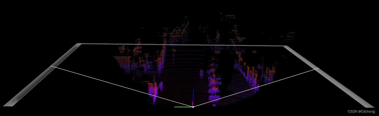
4. Lidar绘制前视图(FOV)+3d box
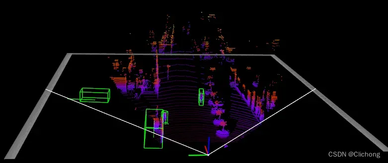
核心是需要将标注框与其方向向量由相机的坐标系中转化到点云的坐标系中进行可视化,在点云空间中绘制3d边界框实现上与在图像上绘制3d框投影类似。
def show_lidar_with_boxes(
    pc_velo,
    objects,
    calib,
    img_fov=False,
    img_width=None,
    img_height=None,
    objects_pred=None,
    depth=None,
    cam_img=None,
):
    """ Show all LiDAR points.
        Draw 3d box in LiDAR point cloud (in velo coord system) """
    if "mlab" not in sys.modules:
        import mayavi.mlab as mlab
    from viz_util import draw_lidar_simple, draw_lidar, draw_gt_boxes3d

    print(("All point num: ", pc_velo.shape[0]))
    fig = mlab.figure(  # 大小颜色设置
        figure=None, bgcolor=(0, 0, 0), fgcolor=None, engine=None, size=(1000, 500)
    )
    if img_fov:
        pc_velo = get_lidar_in_image_fov(   # 获取前视图的点云
            pc_velo[:, 0:3], calib, 0, 0, img_width, img_height
        )
        print(("FOV point num: ", pc_velo.shape[0]))
    print("pc_velo", pc_velo.shape)
    draw_lidar(pc_velo, fig=fig)    # 显示前视图点云
    # pc_velo=pc_velo[:,0:3]

    color = (0, 1, 0)
    for obj in objects:
        if obj.type == "DontCare":
            continue
        # Draw 3d bounding box
        _, box3d_pts_3d = utils.compute_box_3d(obj, calib.P)            # 得到相机坐标系下的点云数据
        box3d_pts_3d_velo = calib.project_rect_to_velo(box3d_pts_3d)    # 将3d标注框转换到原始点云坐标系中

        # 对当前对象绘制3d标注框
        draw_gt_boxes3d([box3d_pts_3d_velo], fig=fig, color=color)
        ......

        # Draw heading arrow 绘制方向
        _, ori3d_pts_3d = utils.compute_orientation_3d(obj, calib.P)    # 获得相机坐标系下的方向向量
        ori3d_pts_3d_velo = calib.project_rect_to_velo(ori3d_pts_3d)    # 将详细坐标系下的向量转化为点云坐标系
        x1, y1, z1 = ori3d_pts_3d_velo[0, :]
        x2, y2, z2 = ori3d_pts_3d_velo[1, :]
        mlab.plot3d(    # 绘制出每个物体的方向
            [x1, x2],
            [y1, y2],
            [z1, z2],
            color=color,
            tube_radius=None,
            line_width=1,
            figure=fig,
        )
        ......
    mlab.show(1)

def draw_gt_boxes3d(
    gt_boxes3d,
    fig,
    color=(1, 1, 1),
    line_width=1,
    draw_text=True,
    text_scale=(1, 1, 1),
    color_list=None,
    label=""
):
    num = len(gt_boxes3d)
    for n in range(num):    # 列表中一般只有一个GT
        b = gt_boxes3d[n]
        if color_list is not None:
            color = color_list[n]
        if draw_text:
            mlab.text3d(
                b[4, 0],
                b[4, 1],
                b[4, 2],
                label,
                scale=text_scale,
                color=color,
                figure=fig,
            )
        # 在点云空间中逆时针依次划线绘制3d标注框
        for k in range(0, 4):
            # http://docs.enthought.com/mayavi/mayavi/auto/mlab_helper_functions.html
            i, j = k, (k + 1) % 4
            mlab.plot3d(    # 依次画顶
                [b[i, 0], b[j, 0]],
                [b[i, 1], b[j, 1]],
                [b[i, 2], b[j, 2]],
                color=color,
                tube_radius=None,
                line_width=line_width,
                figure=fig,
            )

            i, j = k + 4, (k + 1) % 4 + 4
            mlab.plot3d(    # 画竖线
                [b[i, 0], b[j, 0]],
                [b[i, 1], b[j, 1]],
                [b[i, 2], b[j, 2]],
                color=color,
                tube_radius=None,
                line_width=line_width,
                figure=fig,
            )

            i, j = k, k + 4
            mlab.plot3d(    # 画底面
                [b[i, 0], b[j, 0]],
                [b[i, 1], b[j, 1]],
                [b[i, 2], b[j, 2]],
                color=color,
                tube_radius=None,
                line_width=line_width,
                figure=fig,
            )
    # mlab.show(1)
    # mlab.view(azimuth=180, elevation=70, focalpoint=[ 12.0909996 , -1.04700089, -2.03249991], distance=62.0, figure=fig)
    return fig
5. Lidar绘制鸟瞰图(BEV)
将点云转化为鸟瞰图的核心是弄清楚点云坐标系与图像坐标系的转化。对于图像的坐标轴的原点是位于左上角的,向左是x轴向下是y轴。而点云的坐标轴是前x-左y-上z,如下图所示。也就是说图像坐标系的xy轴与点云的xy轴是正好相反的,弄清楚这个就可以弄清楚代码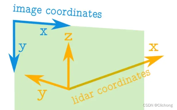
详细解析见:处理点云数据(一):点云与生成鸟瞰图
import numpy as np


# ==============================================================================
#                                                                   SCALE_TO_255
# ==============================================================================
def scale_to_255(a, min, max, dtype=np.uint8):
    """ Scales an array of values from specified min, max range to 0-255
        Optionally specify the data type of the output (default is uint8)
    """
    return (((a - min) / float(max - min)) * 255).astype(dtype)


# ==============================================================================
#                                                         POINT_CLOUD_2_BIRDSEYE
# ==============================================================================
def point_cloud_2_birdseye(points,
                           res=0.1,
                           side_range=(-10., 10.),  # left-most to right-most
                           fwd_range = (-10., 10.), # back-most to forward-most
                           height_range=(-2., 2.),  # bottom-most to upper-most
                           ):
    """ Creates an 2D birds eye view representation of the point cloud data.

    Args:
        points:     (numpy array)
                    N rows of points data
                    Each point should be specified by at least 3 elements x,y,z
        res:        (float)
                    Desired resolution in metres to use. Each output pixel will
                    represent an square region res x res in size.
        side_range: (tuple of two floats)
                    (-left, right) in metres
                    left and right limits of rectangle to look at.
        fwd_range:  (tuple of two floats)
                    (-behind, front) in metres
                    back and front limits of rectangle to look at.
        height_range: (tuple of two floats)
                    (min, max) heights (in metres) relative to the origin.
                    All height values will be clipped to this min and max value,
                    such that anything below min will be truncated to min, and
                    the same for values above max.
    Returns:
        2D numpy array representing an image of the birds eye view.
    """
    # EXTRACT THE POINTS FOR EACH AXIS
    x_points = points[:, 0]
    y_points = points[:, 1]
    z_points = points[:, 2]

    # FILTER - To return only indices of points within desired cube
    # Three filters for: Front-to-back, side-to-side, and height ranges
    # Note left side is positive y axis in LIDAR coordinates
    f_filt = np.logical_and((x_points > fwd_range[0]), (x_points < fwd_range[1]))
    s_filt = np.logical_and((y_points > -side_range[1]), (y_points < -side_range[0]))
    filter = np.logical_and(f_filt, s_filt)
    indices = np.argwhere(filter).flatten()

    # KEEPERS
    x_points = x_points[indices]
    y_points = y_points[indices]
    z_points = z_points[indices]

    # CONVERT TO PIXEL POSITION VALUES - Based on resolution
    x_img = (-y_points / res).astype(np.int32)  # x axis is -y in LIDAR
    y_img = (-x_points / res).astype(np.int32)  # y axis is -x in LIDAR

    # SHIFT PIXELS TO HAVE MINIMUM BE (0,0)
    # floor & ceil used to prevent anything being rounded to below 0 after shift
    x_img -= int(np.floor(side_range[0] / res))
    y_img += int(np.ceil(fwd_range[1] / res))

    # CLIP HEIGHT VALUES - to between min and max heights
    pixel_values = np.clip(a=z_points,
                           a_min=height_range[0],
                           a_max=height_range[1])

    # RESCALE THE HEIGHT VALUES - to be between the range 0-255
    pixel_values = scale_to_255(pixel_values,
                                min=height_range[0],
                                max=height_range[1])

    # INITIALIZE EMPTY ARRAY - of the dimensions we want
    x_max = 1 + int((side_range[1] - side_range[0]) / res)
    y_max = 1 + int((fwd_range[1] - fwd_range[0]) / res)
    im = np.zeros([y_max, x_max], dtype=np.uint8)

    # FILL PIXEL VALUES IN IMAGE ARRAY
    im[y_img, x_img] = pixel_values

    return im
6. Lidar绘制鸟瞰图(BEV)+2d box
- 2d box展示:
- 3d box展示:
以上两幅是一组的,一个鸟瞰图标注,一个点云标注。核心只是在第5节中,在点云投影到鸟瞰图时顺便将3d的标注框也投影到鸟瞰图中。而且鸟瞰图是不需要z轴信息,所以直接使用4个点的xy即可描绘鸟瞰图的2d标注,代码在上诉基础上稍微改进如下:
def point_cloud_2_birdseye_with_2d_bbox(points,
                                        gt,
                                        res=0.1,
                                        side_range=(-40., 40.),  # left-most to right-most
                                        fwd_range=(-70., 70.),   # back-most to forward-most
                                        height_range=(-2., 2.),  # bottom-most to upper-most
                                        ):
    """ Creates an 2D birds eye view representation of the point cloud data.

    Args:
        points:     (numpy array)
                    N rows of points data
                    Each point should be specified by at least 3 elements x,y,z
        res:        (float)
                    Desired resolution in metres to use. Each output pixel will
                    represent an square region res x res in size.
        side_range: (tuple of two floats)
                    (-left, right) in metres
                    left and right limits of rectangle to look at.
        fwd_range:  (tuple of two floats)
                    (-behind, front) in metres
                    back and front limits of rectangle to look at.
        height_range: (tuple of two floats)
                    (min, max) heights (in metres) relative to the origin.
                    All height values will be clipped to this min and max value,
                    such that anything below min will be truncated to min, and
                    the same for values above max.
    Returns:
        2D numpy array representing an image of the birds eye view.
    """
    # EXTRACT THE POINTS FOR EACH AXIS
    x_points = points[:, 0]
    y_points = points[:, 1]
    z_points = points[:, 2]

    # FILTER - To return only indices of points within desired cube
    # Three filters for: Front-to-back, side-to-side, and height ranges
    # Note left side is positive y axis in LIDAR coordinates
    f_filt = np.logical_and((x_points > fwd_range[0]), (x_points < fwd_range[1]))
    s_filt = np.logical_and((y_points > -side_range[1]), (y_points < -side_range[0]))
    filter = np.logical_and(f_filt, s_filt)
    indices = np.argwhere(filter).flatten()

    # KEEPERS
    x_points = x_points[indices]
    y_points = y_points[indices]
    z_points = z_points[indices]

    # GT
    x_gt = gt[..., 0]
    y_gt = gt[..., 1]

    # CONVERT TO PIXEL POSITION VALUES - Based on resolution
    x_img = (-y_points / res).astype(np.int32)  # x axis is -y in LIDAR
    y_img = (-x_points / res).astype(np.int32)  # y axis is -x in LIDAR
    x_bbox = (-y_gt / res).astype(np.int32)
    y_bbox = (-x_gt / res).astype(np.int32)

    # SHIFT PIXELS TO HAVE MINIMUM BE (0,0)
    # floor & ceil used to prevent anything being rounded to below 0 after shift
    x_img -= int(np.floor(side_range[0] / res))
    y_img += int(np.ceil(fwd_range[1] / res))
    x_bbox -= int(np.floor(side_range[0] / res))
    y_bbox += int(np.ceil(fwd_range[1] / res))

    # CLIP HEIGHT VALUES - to between min and max heights
    pixel_values = np.clip(a=z_points,
                           a_min=height_range[0],
                           a_max=height_range[1])

    # RESCALE THE HEIGHT VALUES - to be between the range 0-255
    pixel_values = scale_to_255(pixel_values,
                                min=height_range[0],
                                max=height_range[1])

    # INITIALIZE EMPTY ARRAY - of the dimensions we want
    x_max = int((side_range[1] - side_range[0]) / res) + 1
    y_max = int((fwd_range[1] - fwd_range[0]) / res) + 1
    im = np.zeros([y_max, x_max], dtype=np.uint8)

    # FILL PIXEL VALUES IN IMAGE ARRAY
    im[y_img, x_img] = pixel_values
    bboxes = (y_bbox, x_bbox)

    return im, bboxes


def bbox3d(obj, calib):
    _, box3d_pts_3d = utils.compute_box_3d(obj, calib.P)
    box3d_pts_3d_velo = calib.project_rect_to_velo(box3d_pts_3d)    # 投影到点云坐标系中
    return box3d_pts_3d_velo


def draw_2d_bbox(img, bbox):
    from PIL import ImageDraw, Image
    y_bbox, x_bbox = bbox
    img = np.dstack((img, img, img)).astype(np.uint8)
    img = Image.fromarray(img)
    draw = ImageDraw.Draw(img)
    for x, y in zip(x_bbox, y_bbox):
        x_min = x.min()
        x_max = x.max()
        y_min = y.min()
        y_max = y.max()
        draw.rectangle([x_min,y_min,x_max,y_max], outline=(255, 0, 0))   # 首先要确保img是三个通道的
    img.show()


if __name__ == '__main__':
    # kitti_file = r'E:\Study\Machine Learning\Dataset3d\kitti\training\velodyne\000100.bin'
    # pointcloud = np.fromfile(file=kitti_file, dtype=np.float32, count=-1).reshape([-1, 4])
    # img = point_cloud_2_birdseye(pointcloud)
    # img = Image.fromarray(img)
    # img.show()

    from kitti_object import kitti_object
    root_dir = r'E:\Study\Machine Learning\Dataset3d\kitti'
    data_idx = 2
    dataset = kitti_object(root_dir=root_dir)
    objects = dataset.get_label_objects(data_idx)
    calib = dataset.get_calibration(data_idx)
    pc_velo = dataset.get_lidar(data_idx)[:, 0:4]

    boxes3d = [bbox3d(obj, calib) for obj in objects if obj.type != "DontCare"]
    gt = np.array(boxes3d)
    top_image, bboxes = point_cloud_2_birdseye_with_2d_bbox(pc_velo, gt)    # 将标注框也进行鸟瞰图投影
    draw_2d_bbox(top_image, bboxes)
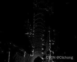
7. Lidar绘制全景图(RV)
什么是RV,RV是Range View,RV是将三维空间中的点投影到可以展开的圆柱形表面上,以将其平面化。先看看3d场景图:
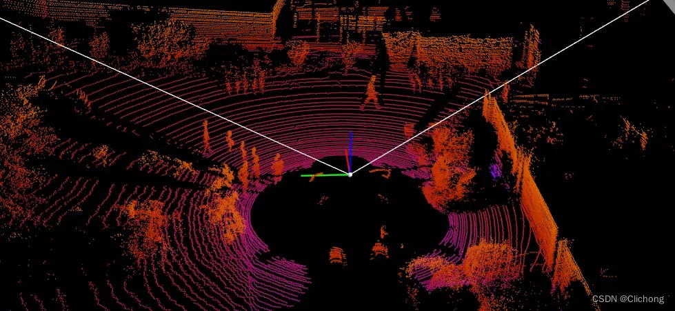
激光雷达的点云来自于多条激光扫描线。比如说64线的激光雷达,那么在垂直方向(Inclination)上就有64个离散的角度。激光雷达在FOV内扫描一遍,会有多个水平方向(Azimuth)的角度。比如说水平分辨率是0.2°,那么扫描360°就会产生1800个离散的角度。这里也可以粗略把Inclination和Azimuth理解为地球上的纬度和经度。把水平和垂直方向的角度值作为X-Y坐标,就可以得到一个二维图像。


图像中的像素值是相应角度下的反射点的特性,比如距离,反射强度等。这些特性可以作为图像的channel,类似于可见光图像中的RGB。如上图所示,分别就对应着depth、height、reflectance三种不同特性所生成的全景图。
ps:这里需要对y坐标进行取反以进行方向上的匹配
- 用matplotlib实现代码:
def lidar_to_2d_front_view(points,
                           v_res=0.4,
                           h_res=0.35,
                           v_fov=(-24.9, 2.0),
                           val="depth",
                           cmap="jet",
                           saveto=None,
                           y_fudge=5
                           ):
    """ Takes points in 3D space from LIDAR data and projects them to a 2D
        "front view" image, and saves that image.

    Args:
        points: (np array)
            The numpy array containing the lidar points.
            The shape should be Nx4
            - Where N is the number of points, and
            - each point is specified by 4 values (x, y, z, reflectance)
        v_res: (float)
            激光雷达的垂直分辨率: 垂直视角为26.9度,分辨率为0.4度
            vertical resolution of the lidar sensor used.
        h_res: (float)
            激光雷达的水平分辨率: 360度的水平视野,分辨率为0.08-0.35(取决于旋转速度)
            horizontal resolution of the lidar sensor used.
        v_fov: (tuple of two floats)
            垂直视野被分成传感器上方+2度和传感器下方-24.9度
            (minimum_negative_angle, max_positive_angle)
        val: (str)
            What value to use to encode the points that get plotted.
            One of {"depth", "height", "reflectance"}
        cmap: (str)
            Color map to use to color code the `val` values.
            NOTE: Must be a value accepted by matplotlib's scatter function
            Examples: "jet", "gray"
        saveto: (str or None)
            If a string is provided, it saves the image as this filename.
            If None, then it just shows the image.
        y_fudge: (float)
            A hacky fudge factor to use if the theoretical calculations of
            vertical range do not match the actual data.

            For a Velodyne HDL 64E, set this value to 5.
    """

    # DUMMY PROOFING
    assert len(v_fov) == 2, "v_fov must be list/tuple of length 2"
    assert v_fov[0] <= 0, "first element in v_fov must be 0 or negative"
    assert val in {"depth", "height", "reflectance"}, \
        'val must be one of {"depth", "height", "reflectance"}'

    # 分别获取点云的xyz坐标以及反射强度
    x_lidar = points[:, 0]
    y_lidar = points[:, 1]
    z_lidar = points[:, 2]
    r_lidar = points[:, 3]  # Reflectance
    # Distance relative to origin when looked from top
    d_lidar = np.sqrt(x_lidar ** 2 + y_lidar ** 2)
    # Absolute distance relative to origin
    # d_lidar = np.sqrt(x_lidar ** 2 + y_lidar ** 2, z_lidar ** 2)

    v_fov_total = -v_fov[0] + v_fov[1]

    # Convert to Radians 转换为弧度
    v_res_rad = v_res * (np.pi/180)
    h_res_rad = h_res * (np.pi/180)

    # PROJECT INTO IMAGE COORDINATES 投影到图像坐标
    x_img = np.arctan2(-y_lidar, x_lidar)/ h_res_rad    # 由于kitti坐标系问题需要对y取反
    y_img = np.arctan2(z_lidar, d_lidar)/ v_res_rad

    # SHIFT COORDINATES TO MAKE 0,0 THE MINIMUM 转换坐标使得(0,0)是最小的
    x_min = -360.0 / h_res / 2  # Theoretical min x value based on sensor specs
    x_img -= x_min              # Shift
    x_max = 360.0 / h_res       # Theoretical max x value after shifting

    y_min = v_fov[0] / v_res    # theoretical min y value based on sensor specs
    y_img -= y_min              # Shift
    y_max = v_fov_total / v_res # Theoretical max x value after shifting

    y_max += y_fudge            # Fudge factor if the calculations based on
                                # spec sheet do not match the range of
                                # angles collected by in the data.

    # WHAT DATA TO USE TO ENCODE THE VALUE FOR EACH PIXEL
    if val == "reflectance":
        pixel_values = r_lidar    # 使用反射强度进行编码
    elif val == "height":
        pixel_values = z_lidar    # 使用高度信息进行编码
    else:
        pixel_values = -d_lidar   # 使用深度信息进行编码

    # PLOT THE IMAGE
    cmap = "jet"            # Color map to use
    dpi = 100               # Image resolution
    fig, ax = plt.subplots(figsize=(x_max/dpi, y_max/dpi), dpi=dpi)
    ax.scatter(x_img, y_img, s=1, c=pixel_values, linewidths=0, alpha=1, cmap=cmap)
    # ax.set_axis_bgcolor((0, 0, 0)) # Set regions with no points to black
    ax.axis('scaled')              # {equal, scaled}
    ax.xaxis.set_visible(False)    # Do not draw axis tick marks
    ax.yaxis.set_visible(False)    # Do not draw axis tick marks
    plt.xlim([0, x_max])   # prevent drawing empty space outside of horizontal FOV
    plt.ylim([0, y_max])   # prevent drawing empty space outside of vertical FOV

    if saveto is not None:
        fig.savefig(saveto, dpi=dpi, bbox_inches='tight', pad_inches=0.0)
    else:
        fig.show()


if __name__ == '__main__':
    kitti_file = r'E:\Study\Machine Learning\Dataset3d\kitti\training\velodyne\000100.bin'
    points = np.fromfile(file=kitti_file, dtype=np.float32, count=-1).reshape([-1, 4])

    HRES = 0.35  # horizontal resolution (assuming 20Hz setting)
    VRES = 0.4  # vertical res
    VFOV = (-24.9, 2.0)  # Field of view (-ve, +ve) along vertical axis
    Y_FUDGE = 5  # y fudge factor for velodyne HDL 64E

    lidar_to_2d_front_view(points, v_res=VRES, h_res=HRES, v_fov=VFOV, val="depth",
                           saveto="E:\\workspace\\PointCloud\\kitti_object_vis\\tmp\\lidar_depth.png", y_fudge=Y_FUDGE)
    lidar_to_2d_front_view(points, v_res=VRES, h_res=HRES, v_fov=VFOV, val="height",
                           saveto="E:\\workspace\\PointCloud\\kitti_object_vis\\tmp\\lidar_height.png", y_fudge=Y_FUDGE)
    lidar_to_2d_front_view(points, v_res=VRES, h_res=HRES, v_fov=VFOV, val="reflectance",
                           saveto="E:\\workspace\\PointCloud\\kitti_object_vis\\tmp\\lidar_reflectance.png",
                           y_fudge=Y_FUDGE)
- 用numpy实现代码:

效果图如上
# ==============================================================================
#                                                                   SCALE_TO_255
# ==============================================================================
def scale_to_255(a, min, max, dtype=np.uint8):
    """ Scales an array of values from specified min, max range to 0-255
        Optionally specify the data type of the output (default is uint8)
    """
    return (((a - min) / float(max - min)) * 255).astype(dtype)


# ==============================================================================
#                                                        POINT_CLOUD_TO_PANORAMA
# ==============================================================================
def point_cloud_to_panorama(points,
                            v_res=0.42,
                            h_res=0.35,
                            v_fov=(-24.9, 2.0),
                            d_range=(0, 100),
                            y_fudge=3
                            ):
    """ Takes point cloud data as input and creates a 360 degree panoramic
        image, returned as a numpy array.

    Args:
        points: (np array)
            The numpy array containing the point cloud. .
            The shape should be at least Nx3 (allowing for more columns)
            - Where N is the number of points, and
            - each point is specified by at least 3 values (x, y, z)
        v_res: (float)
            vertical angular resolution in degrees. This will influence the
            height of the output image.
        h_res: (float)
            horizontal angular resolution in degrees. This will influence
            the width of the output image.
        v_fov: (tuple of two floats)
            Field of view in degrees (-min_negative_angle, max_positive_angle)
        d_range: (tuple of two floats) (default = (0,100))
            Used for clipping distance values to be within a min and max range.
        y_fudge: (float)
            A hacky fudge factor to use if the theoretical calculations of
            vertical image height do not match the actual data.
    Returns:
        A numpy array representing a 360 degree panoramic image of the point
        cloud.
    """
    # Projecting to 2D
    x_points = points[:, 0]
    y_points = points[:, 1]
    z_points = points[:, 2]
    r_points = points[:, 3]
    d_points = np.sqrt(x_points ** 2 + y_points ** 2)  # map distance relative to origin
    #d_points = np.sqrt(x_points**2 + y_points**2 + z_points**2) # abs distance

    # We use map distance, because otherwise it would not project onto a cylinder,
    # instead, it would map onto a segment of slice of a sphere.

    # RESOLUTION AND FIELD OF VIEW SETTINGS
    v_fov_total = -v_fov[0] + v_fov[1]

    # CONVERT TO RADIANS
    v_res_rad = v_res * (np.pi / 180)
    h_res_rad = h_res * (np.pi / 180)

    # MAPPING TO CYLINDER
    x_img = np.arctan2(y_points, x_points) / h_res_rad
    y_img = -(np.arctan2(z_points, d_points) / v_res_rad)

    # THEORETICAL MAX HEIGHT FOR IMAGE
    d_plane = (v_fov_total/v_res) / (v_fov_total* (np.pi / 180))
    h_below = d_plane * np.tan(-v_fov[0]* (np.pi / 180))
    h_above = d_plane * np.tan(v_fov[1] * (np.pi / 180))
    y_max = int(np.ceil(h_below+h_above + y_fudge))

    # SHIFT COORDINATES TO MAKE 0,0 THE MINIMUM
    x_min = -360.0 / h_res / 2
    x_img = np.trunc(-x_img - x_min).astype(np.int32)
    x_max = int(np.ceil(360.0 / h_res))

    y_min = -((v_fov[1] / v_res) + y_fudge)
    y_img = np.trunc(y_img - y_min).astype(np.int32)

    # CLIP DISTANCES
    d_points = np.clip(d_points, a_min=d_range[0], a_max=d_range[1])

    # CONVERT TO IMAGE ARRAY
    img = np.zeros([y_max + 1, x_max + 1], dtype=np.uint8)
    img[y_img, x_img] = scale_to_255(d_points, min=d_range[0], max=d_range[1])

    return img


if __name__ == '__main__':
    kitti_file = r'E:\Study\Machine Learning\Dataset3d\kitti\training\velodyne\000000.bin'
    points = np.fromfile(file=kitti_file, dtype=np.float32, count=-1).reshape([-1, 4])
    img = point_cloud_to_panorama(points)
    img = Image.fromarray(img)
    img.show()
8. Lidar绘制全景图(RV)+2d box

与之前的内容类似,我们可以根据标注信息得到3d的点云坐标,那么对3d点云坐标进行全景图柱坐标系进行投影即可在全景图Range View上进行2d边界框的绘制。核心是获取标注框的3d点云信息,然后对3d点云信息按照相同range view坐标转换即可。
仿照着第六节的信息,参考代码如下:
def point_cloud_to_panorama_with_2d_bbox(points,
                                         gt,
                                         v_res=0.4,
                                         h_res=0.35,
                                         v_fov=(-24.9, 2.0),
                                         val="depth",
                                         y_fudge=5
                                         ):
    """ Takes points in 3D space from LIDAR data and projects them to a 2D
        "front view" image, and saves that image.

    Args:
        points: (np array)
            The numpy array containing the lidar points.
            The shape should be Nx4
            - Where N is the number of points, and
            - each point is specified by 4 values (x, y, z, reflectance)
        v_res: (float)
            激光雷达的垂直分辨率: 垂直视角为26.9度,分辨率为0.4度
            vertical resolution of the lidar sensor used.
        h_res: (float)
            激光雷达的水平分辨率: 360度的水平视野,分辨率为0.08-0.35(取决于旋转速度)
            horizontal resolution of the lidar sensor used.
        v_fov: (tuple of two floats)
            垂直视野被分成传感器上方+2度和传感器下方-24.9度
            (minimum_negative_angle, max_positive_angle)
        val: (str)
            What value to use to encode the points that get plotted.
            One of {"depth", "height", "reflectance"}
        cmap: (str)
            Color map to use to color code the `val` values.
            NOTE: Must be a value accepted by matplotlib's scatter function
            Examples: "jet", "gray"
        saveto: (str or None)
            If a string is provided, it saves the image as this filename.
            If None, then it just shows the image.
        y_fudge: (float)
            A hacky fudge factor to use if the theoretical calculations of
            vertical range do not match the actual data.

            For a Velodyne HDL 64E, set this value to 5.
    """

    # DUMMY PROOFING
    assert len(v_fov) == 2, "v_fov must be list/tuple of length 2"
    assert v_fov[0] <= 0, "first element in v_fov must be 0 or negative"
    assert val in {"depth", "height", "reflectance"}, \
        'val must be one of {"depth", "height", "reflectance"}'

    # 分别获取点云的xyz坐标以及反射强度
    x_lidar = points[:, 0]
    y_lidar = points[:, 1]
    z_lidar = points[:, 2]
    r_lidar = points[:, 3]  # Reflectance
    # Distance relative to origin when looked from top
    d_lidar = np.sqrt(x_lidar ** 2 + y_lidar ** 2)
    # Absolute distance relative to origin
    # d_lidar = np.sqrt(x_lidar ** 2 + y_lidar ** 2, z_lidar ** 2)

    v_fov_total = -v_fov[0] + v_fov[1]

    # gt process
    x_gt = gt[..., 0]
    y_gt = gt[..., 1]
    z_gt = gt[..., 2]
    d_gt = np.sqrt(x_gt ** 2 + y_gt ** 2)

    # Convert to Radians 转换为弧度
    v_res_rad = v_res * (np.pi/180)
    h_res_rad = h_res * (np.pi/180)

    # PROJECT INTO IMAGE COORDINATES 投影到图像坐标
    x_img = np.arctan2(-y_lidar, x_lidar) / h_res_rad    # 由于kitti坐标系问题需要对y取反
    y_img = np.arctan2(z_lidar, d_lidar) / v_res_rad
    x_bbox = np.arctan2(-y_gt, x_gt) / h_res_rad
    y_bbox = np.arctan2(z_gt, d_gt) / v_res_rad

    # SHIFT COORDINATES TO MAKE 0,0 THE MINIMUM 转换坐标使得(0,0)是最小的
    x_min = -360.0 / h_res / 2  # Theoretical min x value based on sensor specs
    x_img -= x_min              # Shift
    x_max = 360.0 / h_res       # Theoretical max x value after shifting

    y_min = v_fov[0] / v_res    # theoretical min y value based on sensor specs
    y_img -= y_min              # Shift
    y_max = v_fov_total / v_res # Theoretical max x value after shifting

    y_max += y_fudge            # Fudge factor if the calculations based on
                                # spec sheet do not match the range of
                                # angles collected by in the data.
    y_img = y_max - y_img       # 需要将图像上下翻转

    # Bbox Shift
    x_bbox -= x_min
    y_bbox -= y_min
    y_bbox = y_max - y_bbox

    # WHAT DATA TO USE TO ENCODE THE VALUE FOR EACH PIXEL
    if val == "reflectance":
        pixel_values = r_lidar
    elif val == "height":
        pixel_values = z_lidar
    else:
        pixel_values = d_lidar   # 使用深度数据编码每个像素的值

    # CLIP DISTANCES
    pixel_values = np.clip(pixel_values, a_min=0, a_max=100)

    img = np.zeros([int(np.ceil(y_max)) + 1, int(np.ceil(x_max)) + 1], dtype=np.uint8)
    y_img = np.trunc(y_img).astype(np.int32)
    x_img = np.trunc(x_img).astype(np.int32)
    img[y_img, x_img] = scale_to_255(pixel_values, 0, 100)

    y_bbox = np.trunc(y_bbox).astype(np.int32)
    x_bbox = np.trunc(x_bbox).astype(np.int32)
    bboxes = (y_bbox, x_bbox)

    return img, bboxes


def bbox3d(obj, calib):
    _, box3d_pts_3d = utils.compute_box_3d(obj, calib.P)
    box3d_pts_3d_velo = calib.project_rect_to_velo(box3d_pts_3d)    # 投影到点云坐标系中
    return box3d_pts_3d_velo


def draw_2d_bbox(img, bbox):
    from PIL import ImageDraw, Image
    y_bbox, x_bbox = bbox
    img = np.dstack((img, img, img)).astype(np.uint8)
    img = Image.fromarray(img)
    draw = ImageDraw.Draw(img)
    for x, y in zip(x_bbox, y_bbox):
        x_min = x.min()
        x_max = x.max()
        y_min = y.min()
        y_max = y.max()
        draw.rectangle([x_min,y_min,x_max,y_max], outline=(255, 0, 0))   # 首先要确保img是三个通道的
    img.show()


if __name__ == '__main__':

    from kitti_object import kitti_object

    root_dir = r'E:\Study\Machine Learning\Dataset3d\kitti'
    data_idx = 0
    dataset = kitti_object(root_dir=root_dir)
    objects = dataset.get_label_objects(data_idx)
    calib = dataset.get_calibration(data_idx)
    pc_velo = dataset.get_lidar(data_idx)[:, 0:4]

    boxes3d = [bbox3d(obj, calib) for obj in objects if obj.type != "DontCare"]
    gt = np.array(boxes3d)
    top_image, bboxes = point_cloud_to_panorama_with_2d_bbox(pc_velo, gt)
    draw_2d_bbox(top_image, bboxes)
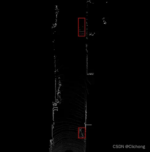
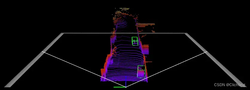
- 测试一:
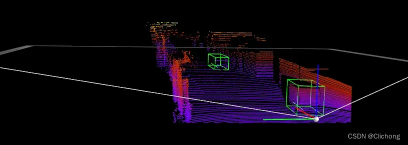
对于全景图的标注信息如果是在远处目标上时,可能标注比较小,难以查看,比如000001.bin点云场景,如下所示,隐隐约约看见远处的3个红色标注框:

其3d场景如图所示,离origin原点处还是比较遥远的:
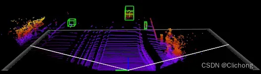
- 测试二:
再来看例外的000002.bin例子:

对应的3d标注是:
参考资料:
- kitti数据集在3D目标检测中的入门(二)可视化详解:https://blog.csdn.net/qq_37534947/article/details/106906219
- 处理点云数据(一):点云与生成鸟瞰图:https://blog.csdn.net/qq_33801763/article/details/78923310
- http://ronny.rest/tutorials/module/pointclouds_01
- http://ronny.rest/blog/post_2017_04_03_point_cloud_panorama/
- KITTI自动驾驶数据集的点云多种视图可视化:https://clichong.blog.csdn.net/article/details/127345052
- kitti_object_vis项目:https://github.com/kuixu/kitti_object_vis
- 激光雷达:最新趋势之基于RangeView的3D物体检测算法:https://zhuanlan.zhihu.com/p/406674156
- 处理点云数据(二):点云与生成前视图:https://blog.csdn.net/qq_33801763/article/details/78924265
- KITTI数据集可视化(一):点云多种视图的可视化实现:https://blog.csdn.net/weixin_44751294/article/details/127345052
文章出处登录后可见!