正在学习人工智能自然语言处理,学校布置的作业分享出来
文章目录
- 1. 原理
- 2. 代码实现
- 2.1.导入的包
- 2.2.分词去停用词
- 2.3.Tfidf
- 2.4.计算困惑度
- 2.5.LDA模型构建
- 2.6.主题与分词
- 2.6.1.权重值
- 2.6.2.每个主题前25个词
- 3.可视化
1. 原理
(参考相关博客与教材)
隐含狄利克雷分布(Latent Dirichlet Allocation,LDA),是一种主题模型(topic model),典型的词袋模型,即它认为一篇文档是由一组词构成的一个集合,词与词之间没有顺序以及先后的关系。一篇文档可以包含多个主题,文档中每一个词都由其中的一个主题生成。它可以将文档集中每篇文档的主题按照概率分布的形式给出,对文章进行主题归纳,属于无监督学习。
需要区分的是,另外一种经典的降维方法线性判别分析(Linear Discriminant Analysis, 简称也为LDA)。此LDA在模式识别领域(比如人脸识别,舰艇识别等图形图像识别领域)中有非常广泛的应用
LDA在训练时不需要手工标注的训练集,需要的仅仅是文档集以及指定主题的数量k即可。此外LDA的另一个优点则是,对于每一个主题均可找出一些词语来描述它。选择模型中topic的数量——人为设置参数,之后输入的每篇文章都给一个topic的概率 每个topic再给其下单词概率,topic的具体实现由自己来定。
LDA 假设文档的生成过程如下:
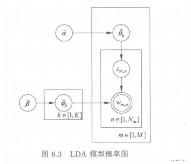
(1)对每个主题:
生成“主题-词项”分布参数: ;(2)对每个文档:生成“文档-主题”分布参数:
;
(3)对当前文档的每个位置。
(a)生成当前位置的所属主题:
;
(b)根据当前位置的主题,以及“主题-词项”分布参数,生成当前位置对应的词项:
2. 代码实现
2.1.导入的包
from matplotlib import pyplot as plt
from sklearn.feature_extraction.text import TfidfTransformer,CountVectorizer
import pandas as pd
import jieba
from sklearn.decomposition import LatentDirichletAllocation
2.2.分词去停用词
with open('train.csv','r',encoding='utf-8') as f:
data = pd.read_csv(f)
# print(data.info())
print(data.content.head())#content列的前5行
with open('中文stopwords.txt','r',encoding='utf-8') as f:
stopwords=[x.strip() for x in f.readlines()]
# print(stopwords[:5])
def cut_stop(content):#分词和去停用词
listx=[]
for row in content:
row=row.replace(" ","")
crow=jieba.lcut(row)
# print(jieba.lcut(row))
for words in crow:
if words in stopwords:
crow.remove(words)
listx.append(crow)
return listx
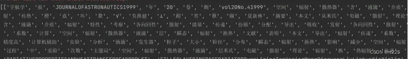
lcontent=cut_stop(data.content[:1000])#生成分词列表
Lcontent[0]:
生成语料
#语料
corpus=[]
for row in lcontent:
text=" ".join(row)
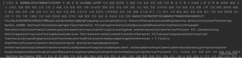
corpus.append(text)
corpus[0]:
2.3.Tfidf
#tfidf
vectorizer = CountVectorizer()
vector=vectorizer.fit_transform(corpus)#转化为词频矩阵
transformer = TfidfTransformer()#该类会统计每个词语的tf-idf权值
tfidf = transformer.fit_transform(vectorizer.fit_transform(corpus))
tfidf_weight = tfidf.toarray()
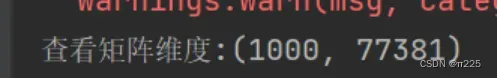
word = vectorizer.get_feature_names()#获取词袋模型中的所有词语
print(f'查看矩阵维度:{vector.shape}')#查看矩阵维度
2.4.计算困惑度
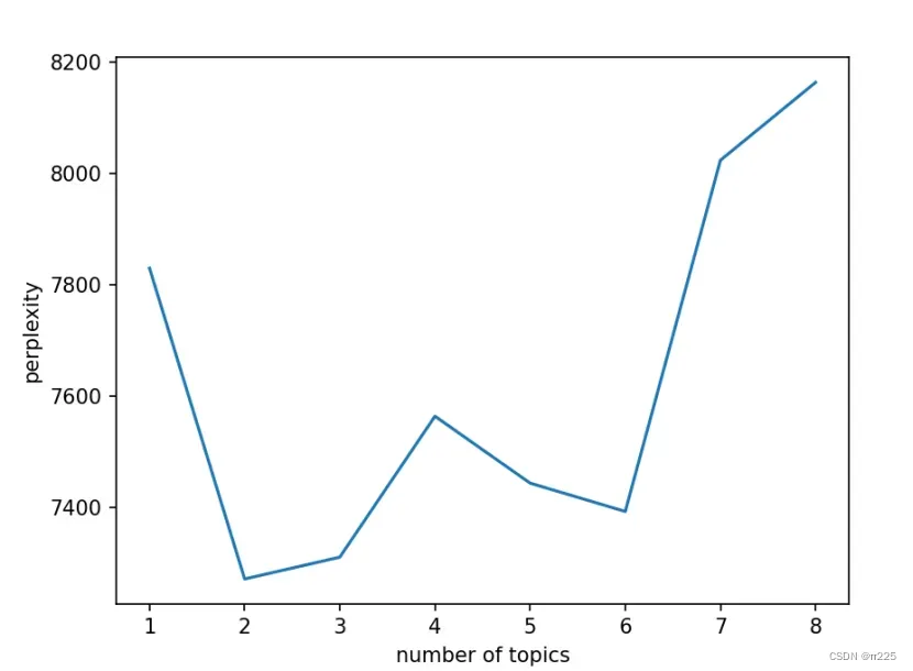
可以简单理解为指定不同聚类数,然后通过lda.perplexity()函数进行处理,或者通过lda.score()进行评分绘制。困惑度理论上选取最低点,或者第一个拐点。绘制可以使用最常用的matplotlib库。
plexs = []
scores = []
n_max_topics = 10
for i in range(1,n_max_topics):
    print('正在进行第',i,'轮计算')
    lda = LatentDirichletAllocation(n_components=i, max_iter=5,
                                    learning_method='online',
                                    learning_offset=50,random_state=0)
    lda.fit(tfidf_weight )
    plexs.append(lda.perplexity(tfidf_weight ))
    scores.append(lda.score(tfidf_weight ))
n_t=9                                      #区间最右侧的值。注意:不能大于等于n_max_topics
x=list(range(1,n_t))
plt.plot(x,plexs[1:n_t])
plt.xlabel("number of topics")
plt.ylabel("perplexity")
plt.show()
见下图,因此选择主题数为2
2.5.LDA模型构建
#LDA构建
n_topics = 2
lda=LatentDirichletAllocation(n_components=n_topics,#主题个数
                              max_iter=5,#EM算法最大迭代次数
                              learning_method='online',#只在fit方法中使用,总体说来,当数据尺寸特别大的时候,在线online更新会比批处理batch更新快得多
                              learning_offset=50.,#一个(正)参数,可以减轻online在线学习中的早期迭代的负担。
                              random_state=0
                              )
lda.fit(tfidf_weight )#拟合
topicc=lda.components_#主题-词项分布
topics=lda.transform(tfidf_weight )#文档-主题分布
2.6.主题与分词
2.6.1.权重值
#每个单词的主题权重值

id = 0
for tt_m in topicc:
    tt_dict = [(name, tt) for name, tt in zip(word, tt_m)]
    tt_dict = sorted(tt_dict, key=lambda x: x[1], reverse=True)
    # 打印权重值大于0.6的主题词:
    # tt_dict = [tt_threshold for tt_threshold in tt_dict if tt_threshold[1] > 0.6]
    # 打印每个类别前5个主题词:
    tt_dict = tt_dict[:8]
    print('主题%d:' % (id), tt_dict)
    id +=1

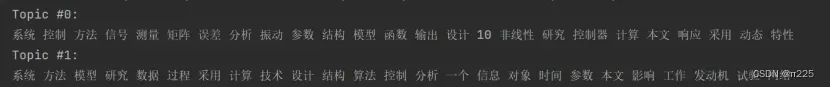
2.6.2.每个主题前25个词
#输出每个主题对应词语
def print_top_words(model, feature_names, n_top_words):
    tword = []
    for topic_idx, topic in enumerate(model.components_):
        print("Topic #%d:" % topic_idx)
        topic_w = " ".join([feature_names[i] for i in topic.argsort()[:-n_top_words - 1:-1]])
        tword.append(topic_w)
        print(topic_w)
    return tword
n_top_words = 25#前几个自己指定
topic_word = print_top_words(lda, word, n_top_words)
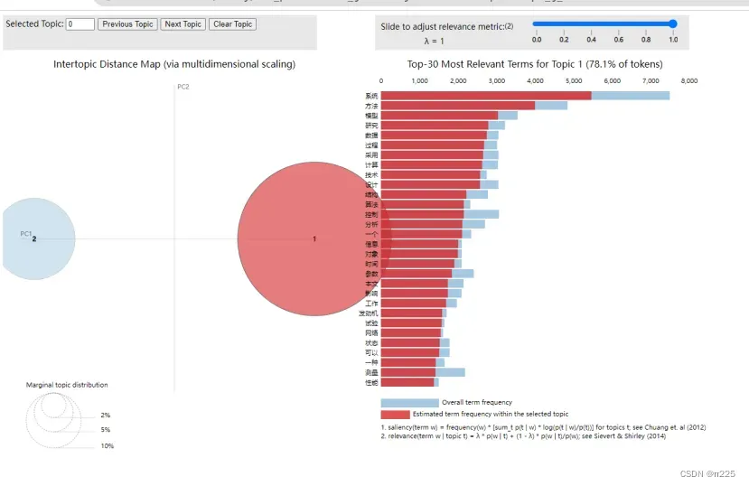
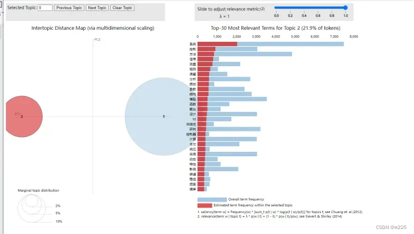
3.可视化
import pyLDAvis.sklearn
pic = pyLDAvis.sklearn.prepare(lda, vector, vectorizer)
pyLDAvis.save_html(pic, 'lda_pass'+str(n_topics)+'.html')
pyLDAvis.show(pic)
文章出处登录后可见!