matplotlib画三维图以及鸢尾花数据进行降维后使用DBSCAN聚类后三维可视化实例

import matplotlib.pyplot as plt
from mpl_toolkits.mplot3d import Axes3D
from sklearn import datasets
from sklearn.decomposition import PCA

iris = datasets.load_iris()
y = iris.target
X_reduced = PCA(n_components=3).fit_transform(iris.data)

fig = plt.figure(1, figsize=(8, 6))
ax = Axes3D(fig, elev=-150, azim=110)

ax.scatter(
    X_reduced[:, 0],
    X_reduced[:, 1],
    X_reduced[:, 2],  # 三维数据
    c=y,  # 数据标签
    cmap=plt.cm.Set1,
    edgecolor="k",
    s=40,
)
ax.set_title("First three PCA directions")
ax.set_xlabel("1st eigenvector")
ax.w_xaxis.set_ticklabels([])
ax.set_ylabel("2nd eigenvector")
ax.w_yaxis.set_ticklabels([])
ax.set_zlabel("3rd eigenvector")
ax.w_zaxis.set_ticklabels([])

plt.show()

运行结果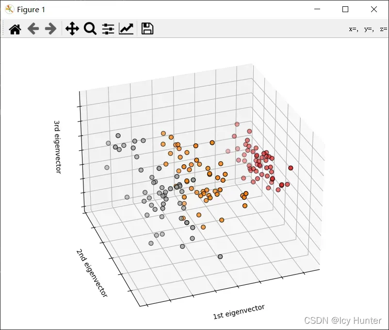

参考：https://scikit-learn.org/stable/auto_examples/datasets/plot_iris_dataset.html#sphx-glr-auto-examples-datasets-plot-iris-dataset-py

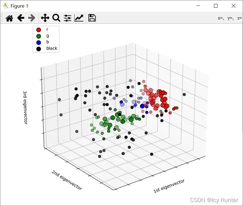
鸢尾花数据进行降维后使用DBSCAN聚类后三维可视化实例

import numpy as np
from sklearn.cluster import DBSCAN
from sklearn import metrics, datasets
from sklearn.decomposition import PCA
from sklearn.preprocessing import StandardScaler
from mpl_toolkits.mplot3d import Axes3D
import matplotlib.pyplot as plt

iris = datasets.load_iris()
labels_true = iris.target
X = PCA(n_components=3).fit_transform(iris.data)
# 数据标准化
X = StandardScaler().fit_transform(X)


# DBSCAN聚类
# eps为邻域半径
# min_samples为确定为核心对象的最小样本数据，即当一个点在他eps半径的区域内共有10个点（包括他自己），那么这个点被确定为核心对象
db = DBSCAN(eps=0.6, min_samples=8).fit(X)
# 找出所有核心点，可视化时图片放大
core_samples_mask = np.zeros_like(db.labels_, dtype=bool)
core_samples_mask[db.core_sample_indices_] = True
labels = db.labels_
# 聚类标签数以及噪声点数
n_clusters_ = len(set(labels)) - (1 if -1 in labels else 0)
n_noise_ = list(labels).count(-1)

print("Estimated number of clusters: %d" % n_clusters_)  # 输出聚类的簇数
print("Estimated number of noise points: %d" % n_noise_)  # 输出噪声点个数

# 需要有正确的标签
print("Homogeneity: %0.3f" % metrics.homogeneity_score(labels_true, labels))  # 同质性homogeneity：每个群集只包含单个类的成员。
print("Completeness: %0.3f" % metrics.completeness_score(labels_true, labels))  # 完整性completeness：给定类的所有成员都分配给同一个群集。
print("V-measure: %0.3f" % metrics.v_measure_score(labels_true, labels))  # 两者的调和平均V-measure：
print("Adjusted Rand Index: %0.3f" % metrics.adjusted_rand_score(labels_true, labels))  # 调整兰德系数，ARI取值范围为[−1,1]，值越大意味着聚类结果与真实情况越吻合。从广义的角度来讲，ARI衡量的是两个数据分布的吻合程度。
print(
    "Adjusted Mutual Information: %0.3f"
    % metrics.adjusted_mutual_info_score(labels_true, labels)
)  # 互信息（Mutual Information）也是用来衡量两个数据分布的吻合程度。利用基于互信息的方法来衡量聚类效果需要实际类别信息，MI与NMI取值范围为[0,1]，AMI取值范围为[−1,1]，它们都是值越大意味着聚类结果与真实情况越吻合。

# 不需要有正确的标签
print("Silhouette Coefficient: %0.3f" % metrics.silhouette_score(X, labels))  # 轮廓系数（Silhouette coefficient）适用于实际类别信息未知的情况。对于一个样本集合，它的轮廓系数是所有样本轮廓系数的平均值。
                                                                              # 轮廓系数取值范围是[−1,1]，同类别样本越距离相近且不同类别样本距离越远，分数越高。


fig = plt.figure(1, figsize=(8, 6))
ax = Axes3D(fig, elev=-150, azim=110)
unique_labels = set(labels)
colors = ["r", "g", "b", "y"]

for k, c in zip(unique_labels, colors):
    if k == -1:
        # Black used for noise.
        c = "black"

    class_member_mask = labels == k

    xy = X[class_member_mask & core_samples_mask]
    ax.scatter(
        xy[:, 0],
        xy[:, 1],
        xy[:, 2],  # 三维数据
        c=c,
        cmap=plt.cm.Set1,
        edgecolor="k",
        s=100,
        label=str(c)
    )

    xy = X[class_member_mask & ~core_samples_mask]
    ax.scatter(
        xy[:, 0],
        xy[:, 1],
        xy[:, 2],  # 三维数据
        c=c,
        cmap=plt.cm.Set1,
        edgecolor="k",
        s=40,
    )
ax.legend(loc="upper left")
xlabel = ["1st eigenvector", "2nd eigenvector", "3rd eigenvector"]
ax.set_title("First three PCA directions")
ax.set_xlabel(xlabel[0])
ax.w_xaxis.set_ticklabels([])
ax.set_ylabel(xlabel[1])
ax.w_yaxis.set_ticklabels([])
ax.set_zlabel(xlabel[2])
ax.w_zaxis.set_ticklabels([])

plt.title("Estimated number of clusters: %d" % n_clusters_)
plt.show()