9 回归问题
9.1 机器学习基础
- 课程回顾
- Python语言基础
- Numpy/Matplotlib/Pandas/Pillow应用
- TensorFlow2.0 低阶API
- 即将学习
- 机器学习、人工神经网络、深度学习、卷积神经网络
- 典型模型的TensorFlow2.0实现
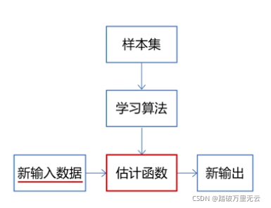
9.1.1 机器学习
- 机器学习(Machine Learning):是通过学习算法从数据中学习模型的过程。
- 过程
- 建立模型 y=wx+b
- 学习模型 确定w,b
- 预测房价 使用模型计算算法
- 学习算法:从数据中产生模型的算法
- 数据集(data set)/样本集(sample set):用来学习的数据的集合
- 样本(sample):数据集中的每一条记录,样本由属性和标定组成
- 属性(attribute):又称为特征(feature):反应样本的表现和性质
- 标记/标签(label):是预测或者分类的结果
9.1.1.1 监督学习(Supervised Learning)
- 监督学习(Supervised Learning):对这种有标记的数据集进行的学习称为监督学习,其过程就是对数据的学习,总结出属性和标签之间的关系,也就是模型。
- 模型/假设(hypothesis)/学习器(learner):估计函数
- 真相/真实(ground truth):学习到的模型应该逼近真正存在的规律
- 监督学习可以分为:
- 回归(regression):预测连续值
- 分类(classfication):预测离散值
9.1.1.2 无监督学习(Unsupervised Learning)
- 无监督学习(Unsupervised Learning):在样本数据没有标记的情况下,挖掘出数据内部蕴含的关系
- 聚类:把相似度高的样本聚合在一起。物以类聚,人以群分,不关心这一类是什么
- 距离:描述了特征值之间的相似度
9.1.1.3 半监督学习(Semi-Supervised Learning)
- 将有监督学习和无监督学习相结合
- 综合使用大量的没有标记数据和少量的有标记数据共同进行学习
9.1.2 机器学习的发展和应用
- 早期机器学习中符号学习是主流、理论研究和模型研究
- 统计机器学习八九十年代发展起来,应用研究
- 机器学习能够抽取出数据中有价值的信息,彰显数据背后的规律,实现大规模的数据识别、分类和预测
9.2 一元线性回归(Simple linear regression)
- y=wx+b
- 模型变量:x
- 模型参数:w为权重(weights)、b为偏置值(bias)
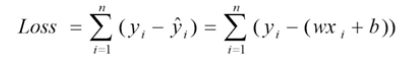
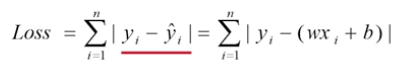
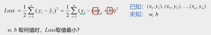
- 估计值:y’i = wxi+b
- 拟合误差/残差:yi-y’i = yi – (wxi+b)
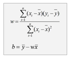
- 最佳拟合直线应该使得所有点的残差累计值最小
9.2.1 损失函数
9.2.1.1 选择损失函数
- 如何做到?
- 残差和最小
损失函数/代价函数(Loss/cast function):模型的预测值和真实值的不一致程度
- 残差绝对值和最小
- 残差平方和最小
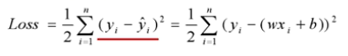
这个loss函数称为平方损失函数(Square Loss),欧氏距离 - 均方误差
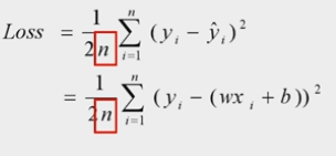
在实际的变成应用中,经常使用它作为损失函数
- 均方误差最小化求解的方法称为最小二乘法(Least Square Method)
9.2.1.2 损失函数的2个性质
- 非负性:保证样本误差不会相互抵消
- 一致性:损失函数的值和误差变化一致。单调有界,收敛于0
9.2.1.3 求解阶段
- 求极值问题:极值点的偏导数为零
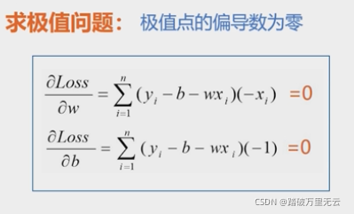
- 求解过程不同,得到的解也可能不同
其实是等价的,一般使用后面的,比较常用
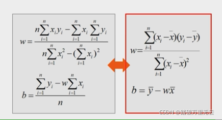
- 通过严格的推到计算得到的解称为解析解(Analytical solution),解析解是一个封闭形式的函数,给出任意自变量,就可以通过严格的公式求出准确的因变量,因此,解析解也被称为封闭解/闭式解(Closed-form solution)
9.3 实例:解析法实现一元线性回归
9.3.1 实例:解析法实现一元线性回归(1)
9.3.1.1 实现一个商品房价值评估系统
- 步骤
- 加载样本数据:x、y
- 学习模型:计算w,b
- 预测房价
y‘ = wx+b
- 下面采用Python、Numpy、TensorFlow来实现
9.3.1.1.1 仅Python实现
9.3.1.1.1.1 加载样本数据
# 1 加载样本数据
x = [137.97,104.50,100.00,124.32,79.20,99.00,124.00,114.00,106.69,138.05,53.75,46.91,68.00,63.02,81.26,86.21]
y = [145.00,110.00,93.00,116.00,65.32,104.00,118.00,91.00,62.00,133.00,51.00,45.00,78.50,69.65,75.69,95.30]
9.3.1.1.1.2 学习模型:计算w,b
# 2 学习模型:计算w,b
meanX = sum(x)/len(x)
meanY = sum(y)/len(y)
sumXY = 0.0
sumY = 0.0
for i in range(len(x)):
    sumXY += (x[i]-meanX)*(y[i]-meanY)
    sumY += (x[i]-meanX)*(x[i]-meanX)
w = sumXY/sumY
b = meanY - w*meanX
print("w=",w)
print("b=",b)
print(type(w),type(b))
输出结果为:
w= 0.8945605120044221
b= 5.410840339418002
<class 'float'> <class 'float'>
9.3.1.1.1.3 预测房价
# 预测房价
x_test = [128.15,45.00,141.43,106.27,99.00,53.84,85.36,70.00]
for i in range(len(x_test)):
    print(x_test[i],"\t",w*x_test[i]+b)
输出结果为:
128.15   120.0487699527847
45.0     45.66606337961699
141.43   131.92853355220342
106.27   100.47578595012793
99.0     93.97233102785579
53.84    53.57397830573609
85.36    81.77052564411547
70.0     68.03007617972756
9.3.1.1.1.4 全部代码记录:
# 1 加载样本数据
x = [137.97,104.50,100.00,124.32,79.20,99.00,124.00,114.00,106.69,138.05,53.75,46.91,68.00,63.02,81.26,86.21]
y = [145.00,110.00,93.00,116.00,65.32,104.00,118.00,91.00,62.00,133.00,51.00,45.00,78.50,69.65,75.69,95.30]
# 2 学习模型:计算w,b
meanX = sum(x)/len(x)
meanY = sum(y)/len(y)
sumXY = 0.0
sumY = 0.0
for i in range(len(x)):
    sumXY += (x[i]-meanX)*(y[i]-meanY)
    sumY += (x[i]-meanX)*(x[i]-meanX)
w = sumXY/sumY
b = meanY - w*meanX
print("w=",w)
print("b=",b)
print(type(w),type(b))
# 预测房价
x_test = [128.15,45.00,141.43,106.27,99.00,53.84,85.36,70.00]
print("面积\t估计房价")
for i in range(len(x_test)):
    print(x_test[i],"\t",round(w*x_test[i]+b,2))
输出结果为:
w= 0.8945605120044221
b= 5.410840339418002
<class 'float'> <class 'float'>
面积    估计房价
128.15   120.05
45.0     45.67
141.43   131.93
106.27   100.48
99.0     93.97
53.84    53.57
85.36    81.77
70.0     68.03
9.3.1.1.2 Numpy实现
9.3.1.1.2.1 加载样本数据
import numpy as np
x = np.array([137.97,104.50,100.00,124.32,79.20,99.00,124.00,114.00,106.69,138.05,53.75,46.91,68.00,63.02,81.26,86.21])
y = np.array([145.00,110.00,93.00,116.00,65.32,104.00,118.00,91.00,62.00,133.00,51.00,45.00,78.50,69.65,75.69,95.30])
9.3.1.1.2.2 学习模型:计算w,b
meanX = np.mean(x)
meanY = np.mean(y)
sumXY = np.sum((x-meanX)*(y-meanY))
sumY = np.sum((x-meanX)*(x-meanX))
w = sumXY/sumY
b = meanY - w*meanX
print("w=",w)
print("b=",b)
print(type(w),type(b))
输出结果为:
w= 0.894560512004422
b= 5.410840339418002
<class 'numpy.float64'> <class 'numpy.float64'>
9.3.1.1.2.3 预测房价
x_test = np.array([128.15,45.00,141.43,106.27,99.00,53.84,85.36,70.00])
y_pred = w*x_test + b
print("面积\t估计房价")
for i in range(len(x_test)):
    print(x_test[i],"\t",np.round(y_pred[i],2))
输出结果为:
面积    估计房价
128.15   120.05
45.0     45.67
141.43   131.93
106.27   100.48
99.0     93.97
53.84    53.57
85.36    81.77
70.0     68.03
9.3.1.1.2.4 代码记录全部
import numpy as np
x = np.array([137.97,104.50,100.00,124.32,79.20,99.00,124.00,114.00,106.69,138.05,53.75,46.91,68.00,63.02,81.26,86.21])
y = np.array([145.00,110.00,93.00,116.00,65.32,104.00,118.00,91.00,62.00,133.00,51.00,45.00,78.50,69.65,75.69,95.30])
meanX = np.mean(x)
meanY = np.mean(y)
sumXY = np.sum((x-meanX)*(y-meanY))
sumY = np.sum((x-meanX)*(x-meanX))
w = sumXY/sumY
b = meanY - w*meanX
print("w=",w)
print("b=",b)
print(type(w),type(b))
x_test = np.array([128.15,45.00,141.43,106.27,99.00,53.84,85.36,70.00])
y_pred = w*x_test + b
print("面积\t估计房价")
for i in range(len(x_test)):
    print(x_test[i],"\t",np.round(y_pred[i],2))
输出结果为:
w= 0.894560512004422
b= 5.410840339418002
<class 'numpy.float64'> <class 'numpy.float64'>
面积    估计房价
128.15   120.05
45.0     45.67
141.43   131.93
106.27   100.48
99.0     93.97
53.84    53.57
85.36    81.77
70.0     68.03
9.3.1.1.3 Tensorflow实现
9.3.1.1.3.1 加载样本数据
import tensorflow as tf
x = tf.constant([137.97,104.50,100.00,124.32,79.20,99.00,124.00,114.00,106.69,138.05,53.75,46.91,68.00,63.02,81.26,86.21])
y = tf.constant([145.00,110.00,93.00,116.00,65.32,104.00,118.00,91.00,62.00,133.00,51.00,45.00,78.50,69.65,75.69,95.30])
9.3.1.1.3.2 学习模型:计算w,b
meanX = tf.reduce_mean(x)
meanY = tf.reduce_mean(y)
sumXY = tf.reduce_sum((x-meanX)*(y-meanY))
sumY = tf.reduce_sum((x-meanX)*(x-meanX))
w = sumXY/sumY
b = meanY - w*meanX
print("w=",w.numpy())
print("b=",b.numpy())
print(type(w),type(b))
输出结果为:
w= 0.8945604
b= 5.4108505
<class 'tensorflow.python.framework.ops.EagerTensor'> <class 'tensorflow.python.framework.ops.EagerTensor'>
9.3.1.1.3.3 预测房价
x_test = tf.constant([128.15,45.00,141.43,106.27,99.00,53.84,85.36,70.00])
y_pred = w*x_test + b
print(y_pred)
输出结果为:
tf.Tensor(
[120.04876   45.66607  131.92853  100.475784  93.97233   53.573982
  81.77052   68.030075], shape=(8,), dtype=float32)
9.3.1.1.3.4 所有代码
import tensorflow as tf
x = tf.constant([137.97,104.50,100.00,124.32,79.20,99.00,124.00,114.00,106.69,138.05,53.75,46.91,68.00,63.02,81.26,86.21])
y = tf.constant([145.00,110.00,93.00,116.00,65.32,104.00,118.00,91.00,62.00,133.00,51.00,45.00,78.50,69.65,75.69,95.30])
meanX = tf.reduce_mean(x)
meanY = tf.reduce_mean(y)
sumXY = tf.reduce_sum((x-meanX)*(y-meanY))
sumY = tf.reduce_sum((x-meanX)*(x-meanX))
w = sumXY/sumY
b = meanY - w*meanX
print("w=",w.numpy())
print("b=",b.numpy())
print(type(w),type(b))
x_test = tf.constant([128.15,45.00,141.43,106.27,99.00,53.84,85.36,70.00])
y_pred = w*x_test + b
print(y_pred)
输出结果为
w= 0.8945604
b= 5.4108505
<class 'tensorflow.python.framework.ops.EagerTensor'> <class 'tensorflow.python.framework.ops.EagerTensor'>
tf.Tensor(
[120.04876   45.66607  131.92853  100.475784  93.97233   53.573982
  81.77052   68.030075], shape=(8,), dtype=float32)
9.3.2 实例:解析法实现一元线性回归(2)
- 不建议直接使用Python列表进行数组运算
- Numpy和Tensorflow支持对多维数组的高效计算
- Numpy仅支持CPU计算,不支持GPU、TPU运算
- Tensorflow支持CPU、GPU高速运算
- Tensorflow提供了快读搭建复杂模型的高阶API,因此,实际编程中通常使用Tensorflow快速搭建模型,并且利用GPU和TPU资源高速运算,使用Numpy读取和访问数据集,接受从GPU输出的中间结果和最终结果,完成数据交换输入和输出的工作
9.3.2.1 数据和模型可视化
- 综合采用Python、Numpy、Tensorflow、Matplotlib实现这个模型
9.3.2.1.1 完整程序实现
9.3.2.1.1.1 导入库,设置字体
import tensorflow as tf
import numpy as np
import matplotlib.pyplot as plt
plt.rcParams['font.sans-serif'] = ['SimHei']
9.3.2.1.1.2 创建Tensor张量,加载样本数据
x = tf.constant([137.97,104.50,100.00,124.32,79.20,99.00,124.00,114.00,106.69,138.05,53.75,46.91,68.00,63.02,81.26,86.21])
y = tf.constant([145.00,110.00,93.00,116.00,65.32,104.00,118.00,91.00,62.00,133.00,51.00,45.00,78.50,69.65,75.69,95.30])
9.3.2.1.1.3 学习模型-计算w、b
# 3 学习模型-计算w、b
meanX = tf.reduce_mean(x)
meanY = tf.reduce_mean(y)
sumXY = tf.reduce_sum((x-meanX)*(y-meanY))
sumY = tf.reduce_sum((x-meanX)*(x-meanX))
w = sumXY/sumY
b = meanY - w*meanX
print("权值w=",w.numpy(),"\n偏置值b=",b.numpy())
print("线性模型:y=",w.numpy(),"* x + ",b.numpy())
输出结果为:
权值w= 0.8945604
偏置值b= 5.4108505
线性模型:y= 0.8945604 * x +  5.4108505
9.3.2.1.1.4 预测房价
# 4 预测房价
x_test = tf.constant([128.15,45.00,141.43,106.27,99.00,53.84,85.36,70.00])
y_pred = (w*x_test + b).numpy()
print("面积\t估计房价")
n = len(x_test)
for i in range(n):
    print(x_test[i],"\t",round(y_pred[i],2))
输出结果为:
面积    估计房价
tf.Tensor(128.15, shape=(), dtype=float32)       120.05
tf.Tensor(45.0, shape=(), dtype=float32)         45.67
tf.Tensor(141.43, shape=(), dtype=float32)       131.93
tf.Tensor(106.27, shape=(), dtype=float32)       100.48
tf.Tensor(99.0, shape=(), dtype=float32)         93.97
tf.Tensor(53.84, shape=(), dtype=float32)        53.57
tf.Tensor(85.36, shape=(), dtype=float32)        81.77
tf.Tensor(70.0, shape=(), dtype=float32)         68.03
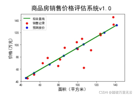
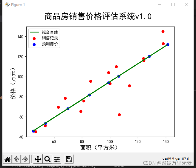
9.3.2.1.1.5 数据和模型可视化
# 5 数据和模型可视化
plt.figure()
plt.scatter(x,y,color="red",label="销售记录")
plt.scatter(x_test,y_pred,color="blue",label="预测房价")
plt.plot(x_test,y_pred,color="green",label="拟合直线",linewidth=2)
plt.xlabel("面积(平方米)",fontsize=14)
plt.ylabel("价格(万元)",fontsize=14)
plt.xlim=(40,150)
plt.ylim=(40,150)
plt.suptitle("商品房销售价格评估系统v1.0",fontsize=20)
plt.legend(loc="upper left")
plt.show()
输出结果为:

9.3.2.1.1.6 本例全部代码
# 1 导入库,设置字体
import tensorflow as tf
import numpy as np
import matplotlib.pyplot as plt
plt.rcParams['font.sans-serif'] = ['SimHei']
# 2 加载样本数据
x = tf.constant([137.97,104.50,100.00,124.32,79.20,99.00,124.00,114.00,106.69,138.05,53.75,46.91,68.00,63.02,81.26,86.21])
y = tf.constant([145.00,110.00,93.00,116.00,65.32,104.00,118.00,91.00,62.00,133.00,51.00,45.00,78.50,69.65,75.69,95.30])
# 3 学习模型-计算w、b
meanX = tf.reduce_mean(x)
meanY = tf.reduce_mean(y)
sumXY = tf.reduce_sum((x-meanX)*(y-meanY))
sumY = tf.reduce_sum((x-meanX)*(x-meanX))
w = sumXY/sumY
b = meanY - w*meanX
print("权值w=",w.numpy(),"\n偏置值b=",b.numpy())
print("线性模型:y=",w.numpy(),"* x + ",b.numpy())
# 4 预测房价
x_test = tf.constant([128.15,45.00,141.43,106.27,99.00,53.84,85.36,70.00])
y_pred = (w*x_test + b).numpy()
print("面积\t估计房价")
n = len(x_test)
for i in range(n):
    print(x_test[i],"\t",round(y_pred[i],2))
# 5 数据和模型可视化
plt.figure()
plt.scatter(x,y,color="red",label="销售记录")
plt.scatter(x_test,y_pred,color="blue",label="预测房价")
plt.plot(x_test,y_pred,color="green",label="拟合直线",linewidth=2)
plt.xlabel("面积(平方米)",fontsize=14)
plt.ylabel("价格(万元)",fontsize=14)
plt.xlim=(40,150)
plt.ylim=(40,150)
plt.suptitle("商品房销售价格评估系统v1.0",fontsize=20)
plt.legend(loc="upper left")
plt.show()
输出结果为:
权值w= 0.8945604
偏置值b= 5.4108505
线性模型:y= 0.8945604 * x +  5.4108505
面积    估计房价
tf.Tensor(128.15, shape=(), dtype=float32)       120.05
tf.Tensor(45.0, shape=(), dtype=float32)         45.67
tf.Tensor(141.43, shape=(), dtype=float32)       131.93
tf.Tensor(106.27, shape=(), dtype=float32)       100.48
tf.Tensor(99.0, shape=(), dtype=float32)         93.97
tf.Tensor(53.84, shape=(), dtype=float32)        53.57
tf.Tensor(85.36, shape=(), dtype=float32)        81.77
tf.Tensor(70.0, shape=(), dtype=float32)         68.03
9.3.3 习题
Tensorflow和Numpy中默认的浮点数类型分别为___A___。
A. float32 float64
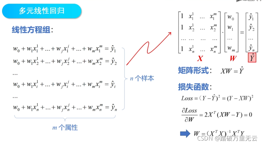
9.4 多元线性回归
- 多元回归(Multivariate Regression):回归分析中包括两个或两个以上的自变量
- 多元线性回归(Multivariate Linear Regression):因变量和自变量之间是线性关系
- 超平面(Hyperplane):直线在高维空间中的推广
- 在本课程中,所有的向量都默认是列向量
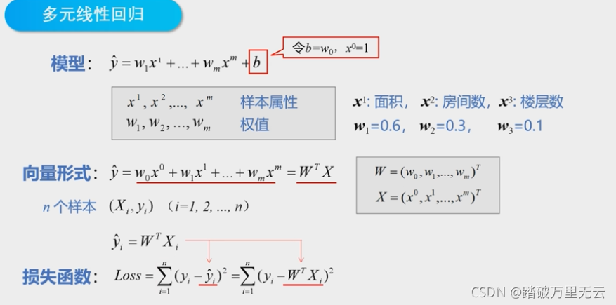
- 损失函数是所有样本误差的平方和
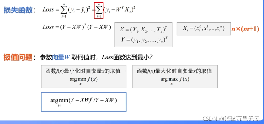
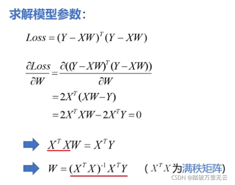
- 使用多元线性回归的时候,直接使用这个解就可以了
- 如果不喜欢向量的形式,也可以使用矩阵的形式
- 使用这种方式求w时,需要对矩阵(XTX)求逆,要求(XTX)结果必须是满秩的,但是现实任务中,它往往不是满秩的;
- 例如,一个样本的属性非常多,甚至超过了样本数,导致x的列数多于行数,这就会使得(XTX)不满秩,在这种情况下,可以解出多个w,它们都能使平方损失函数最小化,造成模型不唯一
- 为了解决这个问题,就需要改变或者调整学习算法,后面的课程中会学习
- 这里的维度概念可能会混淆,但是都是对的
9.5 实例:解析法实现多元线性回归
- 课程回顾

- 例子:仍然使用商品房价格来实验这个
- 多元线性回归分为四步
- 加载样本数据
- 数据处理
- 求解模型参数,学习模型:计算W=(XTX)-1XTY
- 预测房价
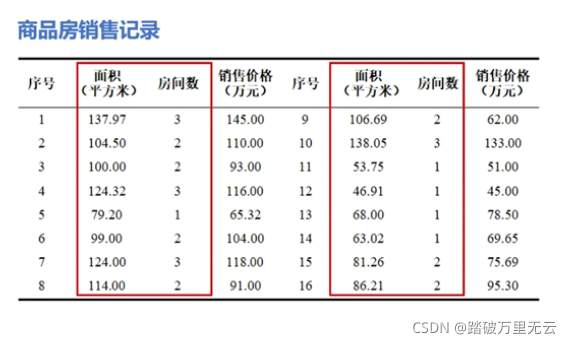
9.5.1 加载样本数据
# 1 加载样本数据
import numpy as np
# 房间面积
x1 = np.array([137.97,104.50,100.00,124.32,79.20,99.00,124.00,114.00,106.69,138.05,53.75,46.91,68.00,63.02,81.26,86.21])
# 房间数
x2 = np.array([3,2,2,3,1,2,3,2,2,3,1,1,1,1,2,2])
# 房价
y = np.array([145.00,110.00,93.00,116.00,65.32,104.00,118.00,91.00,62.00,133.00,51.00,45.00,78.50,69.65,75.69,95.30])
print(x1.shape,x2.shape,y.shape)
输出结果为:
(16,) (16,) (16,)
9.5.2 数据处理
- 将输入的数据处理成模型要求的数据格式
# 2 数据处理
x0 = np.ones(len(x1))
X = np.stack((x0,x1,x2),axis=1)
Y = np.array(y).reshape(-1,1)
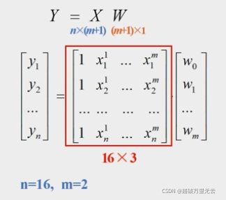
9.5.3 求解模型参数,计算W=(XTX)-1XTY
- W=(XTX)-1XTY
| 功能 | 函数 |
|---|---|
| 矩阵相乘 | np.matmul() |
| 矩阵转置 | np.transpose() |
| 矩阵求逆 | np.linalg.inv() |
# 3 求解模型参数
Xt = np.transpose(X) # 计算X'
XtX_1 = np.linalg.inv(np.matmul(Xt,X)) # 计算(X'X)-1
XtX_1_Xt = np.matmul(XtX_1,Xt) # 计算(X'X)-1X'
W = np.matmul(XtX_1_Xt,Y) # 计算(X'X)-1X'Y
W = W.reshape(-1) # 为了方便后面的引用
print(W)
print("多元线性回归方程:")
print("Y=",W[1]," * x1 + ",W[2]," * x2 + ",W[0])
输出结果为:
[11.96729093  0.53488599 14.33150378]
多元线性回归方程:
Y= [0.53488599]  * x1 +  [14.33150378]  * x2 +  [11.96729093]
9.5.4 预测房价
print("请输入房屋面积和房间数,预测房屋销售价格:")
x1_test=float(input("商品房面积:"))
x2_test=int(input("房间数:"))
y_pred = W[1]*x1_test+W[2]*x2_test+W[0]
print("预测价格:",round(y_pred,2),"万元")
输出结果为:
请输入房屋面积和房间数,预测房屋销售价格:
商品房面积:120
房间数:4
预测价格: 133.48 万元
9.5.5 该例子完整代码
# 1 加载样本数据
import numpy as np
# 房间面积
x1 = np.array([137.97,104.50,100.00,124.32,79.20,99.00,124.00,114.00,106.69,138.05,53.75,46.91,68.00,63.02,81.26,86.21])
# 房间数
x2 = np.array([3,2,2,3,1,2,3,2,2,3,1,1,1,1,2,2])
# 房价
y = np.array([145.00,110.00,93.00,116.00,65.32,104.00,118.00,91.00,62.00,133.00,51.00,45.00,78.50,69.65,75.69,95.30])
print(x1.shape,x2.shape,y.shape)
# 2 数据处理
x0 = np.ones(len(x1))
X = np.stack((x0,x1,x2),axis=1)
Y = np.array(y).reshape(-1,1)
# 3 求解模型参数
Xt = np.transpose(X) # 计算X'
XtX_1 = np.linalg.inv(np.matmul(Xt,X)) # 计算(X'X)-1
XtX_1_Xt = np.matmul(XtX_1,Xt) # 计算(X'X)-1X'
W = np.matmul(XtX_1_Xt,Y) # 计算(X'X)-1X'Y
W = W.reshape(-1) # 为了方便后面的引用
print(W)
print("多元线性回归方程:")
print("Y=",W[1]," * x1 + ",W[2]," * x2 + ",W[0])
print("请输入房屋面积和房间数,预测房屋销售价格:")
x1_test=float(input("商品房面积:"))
x2_test=int(input("房间数:"))
y_pred = W[1]*x1_test+W[2]*x2_test+W[0]
print("预测价格:",round(y_pred,2),"万元")
输出结果为:
(16,) (16,) (16,)
[11.96729093  0.53488599 14.33150378]
多元线性回归方程:
Y= 0.5348859949724712  * x1 +  14.331503777673714  * x2 +  11.96729093053445
请输入房屋面积和房间数,预测房屋销售价格:
商品房面积:120
房间数:4
预测价格: 133.48 万元
9.5.6 Numpy数组运算函数
- 第五讲相似介绍过
| 功能 | 函数 |
|---|---|
| 数组堆叠 | np.stack() |
| 改变数组形状 | np.reshape() |
| 矩阵相乘 | np.matmul() |
| 矩阵转置 | np.transpose() |
| 矩阵求逆 | np.linalg.inv() |
9.6 实例:三维模型可视化
9.6.1 二元线性回归可视化
9.6.1.1 加载数据
# 1 加载样本数据
import numpy as np
import matplotlib.pyplot as plt
from mpl_toolkits.mplot3d import Axes3D
# 房间面积
x1 = np.array([137.97,104.50,100.00,124.32,79.20,99.00,124.00,114.00,106.69,138.05,53.75,46.91,68.00,63.02,81.26,86.21])
# 房间数
x2 = np.array([3,2,2,3,1,2,3,2,2,3,1,1,1,1,2,2])
# 房价
y = np.array([145.00,110.00,93.00,116.00,65.32,104.00,118.00,91.00,62.00,133.00,51.00,45.00,78.50,69.65,75.69,95.30])
W = np.array([11.96729093,0.53488599,14.33150378])
y_pred = W[1]*x1+W[2]*x2+W[0]
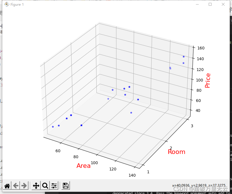
9.6.1.2 绘制散点图
fig = plt.figure(figsize=(8,6))
ax3d = Axes3D(fig)
ax3d.scatter(x1,x2,y,color="b",marker="*")
ax3d.set_xlabel('Area',color='r',fontsize=16)
ax3d.set_ylabel('Room',color='r',fontsize=16)
ax3d.set_zlabel('Price',color='r',fontsize=16)
ax3d.set_yticks([1,2,3]) # 设置y轴的坐标轴刻度,设置的是刻度的显示形式,而不是显示范围
ax3d.set_zlim3d(30,160)
plt.show()
输出结果为:
9.6.1.3 整个代码
# 1 加载样本数据
import numpy as np
import matplotlib.pyplot as plt
from mpl_toolkits.mplot3d import Axes3D
# 房间面积
x1 = np.array([137.97,104.50,100.00,124.32,79.20,99.00,124.00,114.00,106.69,138.05,53.75,46.91,68.00,63.02,81.26,86.21])
# 房间数
x2 = np.array([3,2,2,3,1,2,3,2,2,3,1,1,1,1,2,2])
# 房价
y = np.array([145.00,110.00,93.00,116.00,65.32,104.00,118.00,91.00,62.00,133.00,51.00,45.00,78.50,69.65,75.69,95.30])
W = np.array([11.96729093,0.53488599,14.33150378])
y_pred = W[1]*x1+W[2]*x2+W[0]
fig = plt.figure(figsize=(8,6))
ax3d = Axes3D(fig)
#ax3d.view_init(elev=0,azim=90) # 改变观察视角
ax3d.scatter(x1,x2,y,color="b",marker="*")
ax3d.set_xlabel('Area',color='r',fontsize=16)
ax3d.set_ylabel('Room',color='r',fontsize=16)
ax3d.set_zlabel('Price',color='r',fontsize=16)
ax3d.set_yticks([1,2,3]) # 设置y轴的坐标轴刻度,设置的是刻度的显示形式,而不是显示范围
ax3d.set_zlim3d(30,160)
plt.show()
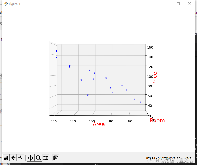
9.6.1.4 改变观察视角
view_init(elev,azim)
- elev:视角的水平高度
- azim:视角的水平旋转的角度
如:
ax3d.view_init(elev=0,azim=90) # 改变观察视角
输出为:
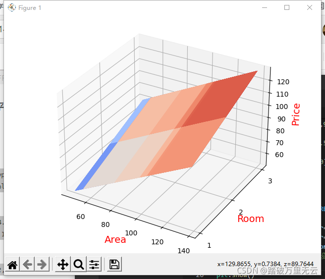
9.6.1.5 绘制平面图
# 1 加载样本数据
import numpy as np
import matplotlib.pyplot as plt
from mpl_toolkits.mplot3d import Axes3D
# 房间面积
x1 = np.array([137.97,104.50,100.00,124.32,79.20,99.00,124.00,114.00,106.69,138.05,53.75,46.91,68.00,63.02,81.26,86.21])
# 房间数
x2 = np.array([3,2,2,3,1,2,3,2,2,3,1,1,1,1,2,2])
# 房价
y = np.array([145.00,110.00,93.00,116.00,65.32,104.00,118.00,91.00,62.00,133.00,51.00,45.00,78.50,69.65,75.69,95.30])
W = np.array([11.96729093,0.53488599,14.33150378])
X1,X2=np.meshgrid(x1,x2) # 生成网格点的坐标矩阵
Y_PRED = W[1]*X1+W[2]*X2+W[0] # 使用模型计算纵坐标
fig = plt.figure()
ax3d = Axes3D(fig)
ax3d.plot_surface(X1,X2,Y_PRED,cmap="coolwarm") # 颜色方案选择coolwarm
ax3d.set_xlabel('Area',color='r',fontsize=14)
ax3d.set_ylabel('Room',color='r',fontsize=14)
ax3d.set_zlabel('Price',color='r',fontsize=14)
ax3d.set_yticks([1,2,3]) # 设置y轴的坐标轴刻度,设置的是刻度的显示形式,而不是显示范围
plt.show()
输出结果为:
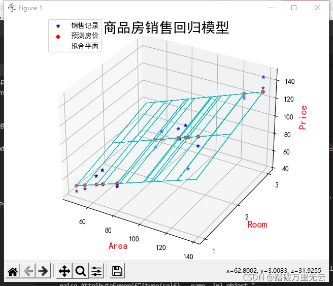
9.6.1.6 绘制散点图和线框图
# 1 加载样本数据
import numpy as np
import matplotlib.pyplot as plt
from mpl_toolkits.mplot3d import Axes3D
# 房间面积
x1 = np.array([137.97,104.50,100.00,124.32,79.20,99.00,124.00,114.00,106.69,138.05,53.75,46.91,68.00,63.02,81.26,86.21])
# 房间数
x2 = np.array([3,2,2,3,1,2,3,2,2,3,1,1,1,1,2,2])
# 房价
y = np.array([145.00,110.00,93.00,116.00,65.32,104.00,118.00,91.00,62.00,133.00,51.00,45.00,78.50,69.65,75.69,95.30])
W = np.array([11.96729093,0.53488599,14.33150378])
y_pred = W[1]*x1+W[2]*x2+W[0] # 使用模型计算纵坐标
plt.rcParams['font.sans-serif'] = ['SimHei']
X1,X2=np.meshgrid(x1,x2) # 生成网格点的坐标矩阵
Y_PRED = W[1]*X1+W[2]*X2+W[0] # 使用模型计算纵坐标
fig = plt.figure()
ax3d = Axes3D(fig)
ax3d.scatter(x1,x2,y,color="b",marker='*',label="销售记录") #实际房价绘制散点图
ax3d.scatter(x1,x2,y_pred,color='r',label="预测房价") # 估计房价绘制散点图
ax3d.plot_wireframe(X1,X2,Y_PRED,color="c",linewidth=0.5,label="拟合平面")
ax3d.set_xlabel('Area',color='r',fontsize=14)
ax3d.set_ylabel('Room',color='r',fontsize=14)
ax3d.set_zlabel('Price',color='r',fontsize=14)
ax3d.set_yticks([1,2,3]) # 设置y轴的坐标轴刻度,设置的是刻度的显示形式,而不是显示范围
plt.suptitle("商品房销售回归模型",fontsize=20)
plt.legend(loc="upper left")
plt.show()
输出结果为:
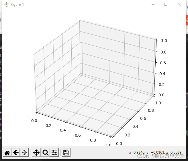
9.6.2 三维数据可视化
9.6.2.1 mplot3d工具集
- 绘制三维图形
- 内置于Matplotlib
- Figure对象
- Axes3d对象;使用之前要导入它
import matplotlib.pyplot as plt
from mpl_toolkits.mplot3d import Axes3D
fig = plt.figure()
ax3d = Axes3D(fig)
plt.show()
输出为:
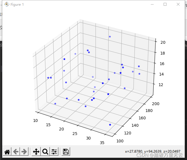
9.6.2.2 绘制散点图–scatter(x,y,z)
import matplotlib.pyplot as plt
from mpl_toolkits.mplot3d import Axes3D
import numpy as np
x = np.random.uniform(10,40,30)
y = np.random.uniform(100,200,30)
z = np.random.uniform(10,20,30)
fig = plt.figure()
ax3d = Axes3D(fig)
ax3d.scatter(x,y,z,c='b',marker="*")
plt.show()
输出结果为:
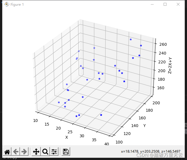
9.6.2.3 绘制散点图–z=2x+y
import matplotlib.pyplot as plt
from mpl_toolkits.mplot3d import Axes3D
import numpy as np
x = np.random.uniform(10,40,30)
y = np.random.uniform(100,200,30)
z = 2*x+y
fig = plt.figure()
ax3d = Axes3D(fig)
ax3d.scatter(x,y,z,c='b',marker="*")
ax3d.set_xlabel('X')
ax3d.set_ylabel('Y')
ax3d.set_zlabel('Z=2X+Y')
plt.show()
输出结果为:
- 还可以绘制平面图、曲面图、线框图,首先要生成平面网格点的坐标矩阵
9.6.2.4 网格点坐标矩阵
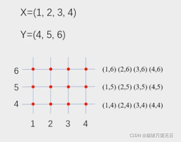
np.meshgrid():生成网格点坐标矩阵
- 接受两个一维数组,生成两个二维数组
>>> import numpy as np
>>> x = [1,2,3,4]
>>> y=[4,5,6]
>>> X,Y=np.meshgrid(x,y)
>>> X
array([[1, 2, 3, 4],
       [1, 2, 3, 4],
       [1, 2, 3, 4]])
>>> Y
array([[4, 4, 4, 4],
       [5, 5, 5, 5],
       [6, 6, 6, 6]])
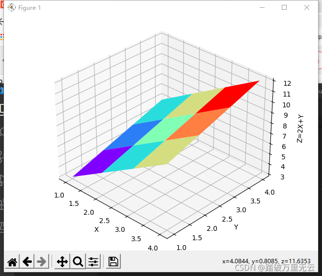
9.6.2.5 绘制平面图–z=2x+y
Axes3D.plot_surface():绘制平面/曲面图
- 测试小代码:
>>> import numpy as np
>>> x = np.arange(1,5)
>>> y = np.arange(1,5)
>>> X,Y=np.meshgrid(x,y)
>>> X.shape
(4, 4)
>>> Y.shape
(4, 4)
>>> Z=2*X+Y
>>> Z.shape
(4, 4)
- 绘制完整代码:
import matplotlib.pyplot as plt
from mpl_toolkits.mplot3d import Axes3D
import numpy as np
x = np.arange(1,5)
y = np.arange(1,5)
X,Y=np.meshgrid(x,y)
Z = 2*X + Y
fig = plt.figure()
ax3d = Axes3D(fig)
ax3d.plot_surface(X,Y,Z,cmap="rainbow")
# 按照彩虹的颜色顺序从高到低排序,Z值大靠近红色,Z值小靠近紫色,颜色相同的色块在同一高度上
# 由于只有4*4个数据,所以划分为3*3的九个格子
ax3d.set_xlabel('X')
ax3d.set_ylabel('Y')
ax3d.set_zlabel('Z=2X+Y')
plt.show()
输出结果为:
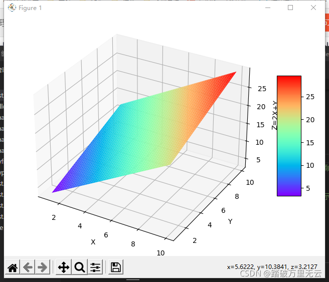
- 可以换成
x = np.arange(1,10)
y = np.arange(1,10)
或
x = np.arange(1,10,0.1)
y = np.arange(1,10,0.1)
试试看
如:
import matplotlib.pyplot as plt
from mpl_toolkits.mplot3d import Axes3D
import numpy as np
x = np.arange(1,10,0.1)
y = np.arange(1,10,0.1)
X,Y=np.meshgrid(x,y)
Z = 2*X + Y
fig = plt.figure()
ax3d = Axes3D(fig)
surf=ax3d.plot_surface(X,Y,Z,cmap="rainbow")
# 按照彩虹的颜色顺序从高到低排序,Z值大靠近红色,Z值小靠近紫色,颜色相同的色块在同一高度上
# 由于只有4*4个数据,所以划分为3*3的九个格子
fig.colorbar(surf,shrink=0.5,aspect=5) # 在图的旁边显示颜色指示条
ax3d.set_xlabel('X')
ax3d.set_ylabel('Y')
ax3d.set_zlabel('Z=2X+Y')
plt.show()
输出结果为:
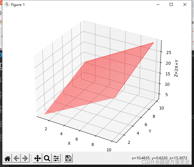
9.6.2.6 绘制线框图–z=2x+y
- 绘制线框图和绘制平民图方式基本完全一样
- 只需要修改绘制函数即可
Axes3D.plot_wireframe()
import matplotlib.pyplot as plt
from mpl_toolkits.mplot3d import Axes3D
import numpy as np
x = np.arange(1,10,0.1)
y = np.arange(1,10,0.1)
X,Y=np.meshgrid(x,y)
Z = 2*X + Y
fig = plt.figure()
ax3d = Axes3D(fig)
ax3d.plot_wireframe(X,Y,Z,color='r',linewidth =0.5)
ax3d.set_xlabel('X')
ax3d.set_ylabel('Y')
ax3d.set_zlabel('Z=2X+Y')
plt.show()
输出结果为:
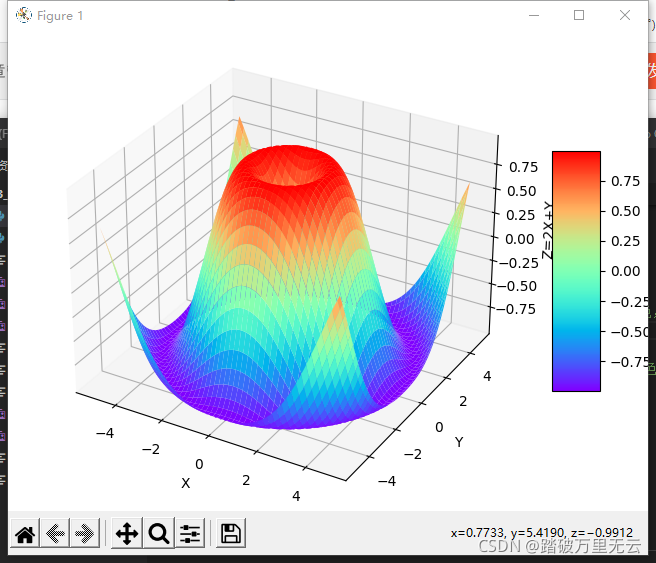
9.6.2.7 绘制曲面图-z=sin(x2+y2)1/2
- 和绘制平面的方法完全一样
- 只要z是一个表示曲面的方程
import matplotlib.pyplot as plt
from mpl_toolkits.mplot3d import Axes3D
import numpy as np
x = np.arange(-5,5,0.1)
y = np.arange(-5,5,0.1)
X,Y=np.meshgrid(x,y)
Z = np.sin(np.sqrt(X**2+Y**2))
fig = plt.figure()
ax3d = Axes3D(fig)
surf=ax3d.plot_surface(X,Y,Z,cmap="rainbow")
# 按照彩虹的颜色顺序从高到低排序,Z值大靠近红色,Z值小靠近紫色,颜色相同的色块在同一高度上
# 由于只有4*4个数据,所以划分为3*3的九个格子
fig.colorbar(surf,shrink=0.5,aspect=5) # 在图的旁边显示颜色指示条
ax3d.set_xlabel('X')
ax3d.set_ylabel('Y')
ax3d.set_zlabel('Z=2X+Y')
plt.show()
输出结果为:
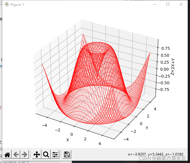
9.6.2.7 绘制曲面线框图-z=sin(x2+y2)1/2
import matplotlib.pyplot as plt
from mpl_toolkits.mplot3d import Axes3D
import numpy as np
x = np.arange(-5,5,0.1)
y = np.arange(-5,5,0.1)
X,Y=np.meshgrid(x,y)
Z = np.sin(np.sqrt(X**2+Y**2))
fig = plt.figure()
ax3d = Axes3D(fig)
ax3d.plot_wireframe(X,Y,Z,color='r',linewidth =0.5)
ax3d.set_xlabel('X')
ax3d.set_ylabel('Y')
ax3d.set_zlabel('Z=2X+Y')
plt.show()
输出结果为:
9.7 参考文献
版权声明:本文为博主踏破万里无云原创文章,遵循 CC 4.0 BY-SA 版权协议,转载请附上原文出处链接和本声明。
原文链接:https://blog.csdn.net/qq_45954434/article/details/121219627