1.总结
预测类数据分析项目
| 流程 | 具体操作 |
|---|---|
| 基本查看 | 查看缺失值(可以用直接查看方式isnull、图像查看方式查看缺失值missingno)、查看数值类型特征与非数值类型特征、一次性绘制所有特征的分布图像 |
| 预处理 | 缺失值处理(填充)拆分数据(获取有需要的值) 、统一数据格式、特征工程(特征编码、0/1字符转换、自定义) 、特征衍生、降维(特征相关性、PCA降维) |
| 数据分析 | groupby分组求最值数据、seaborn可视化 |
| 预测 | 拆分数据集、建立模型(机器学习:RandomForestRegressor、LogisticRegression、GradientBoostingRegressor、RandomForest)、训练模型、预测、评估模型(ROC曲线、MSE、MAE、RMSE、R2)、调参(GridSearchCV) |
数量查看:条形图
占比查看:饼图
数据分区分布查看:概率密度函数图
查看相关关系:条形图、热力图
分布分析:分类直方图(countplot)、分布图-带有趋势线的直方图(distplot)
自然语言处理项目:
| 流程 | 具体操作 |
|---|---|
| 基本查看 | 导入数据 、获取数据转换为列表、 |
| 预处理 | 删除空值、关键词抽取(基于 TF-IDF、基于TextRank )、分词(jieba) 、关键词匹配(词袋模型)、处理分词结果(删除特殊字符、去除停用词) |
| 数据可视化(绘制词云图) | 分组统计数量、训练模型(学习词频信息)、使用自定义背景图、绘制词云图 |
| 建模(文本分类) | 文本分类(LDA模型)、机器学习(朴素贝叶斯)、深度学习(cnn、LSTM、GRU) |
2.项目介绍

前置知识
了解自然语言处理,熟悉相关自然语言处理包,TF-IDF算法、LDA主题模型、CNN、LSTM等深度学习知识
主要内容
- 自然语言处理(NLP)
分词、词袋模型、机器学习、深度学习 - 讲解顺序
词云、文本分析、文本分类
注意
本项目的文本是针对中文处理,所以难度上比英文处理大。因为英文是靠空格分开每个词语,但是中文并没有这样的规律。
3.词云介绍

“词云”就是对文本中出现频率较高的“关键词”予以视觉上的突出,形成“关键词云层”或“关键词渲染”,从而过滤掉大量的文本信息,使浏览者只要一眼扫过文本就可以领略文本的主旨
中文文本处理
- 分词
通过中文分词包进行分词,其中jieba是优秀的中文分词第三方库
安装方式:pip install jieba - 处理分词结果
删除特殊字符、去除停用词等 - 统计词频
- 做词云
wordcloud是优秀的词云展示第三方库,以词语为基本单位,
通过图形可视化的方式,更加直观和艺术的展示文本
安装方式:pip install wordcloud - 自定义背景图做词云
通过imageio读取背景图
安装方式:pip install imageio
4.数据预处理
4.1 分词
import warnings
warnings.filterwarnings("ignore") # 忽略警告信息
import jieba # 分词包
from wordcloud import WordCloud # 词云包
import numpy as np
import pandas as pd
import matplotlib.pyplot as plt
%matplotlib inline
import matplotlib
matplotlib.rcParams['figure.figsize'] = (10.0,5.0)
# 1.读取数据
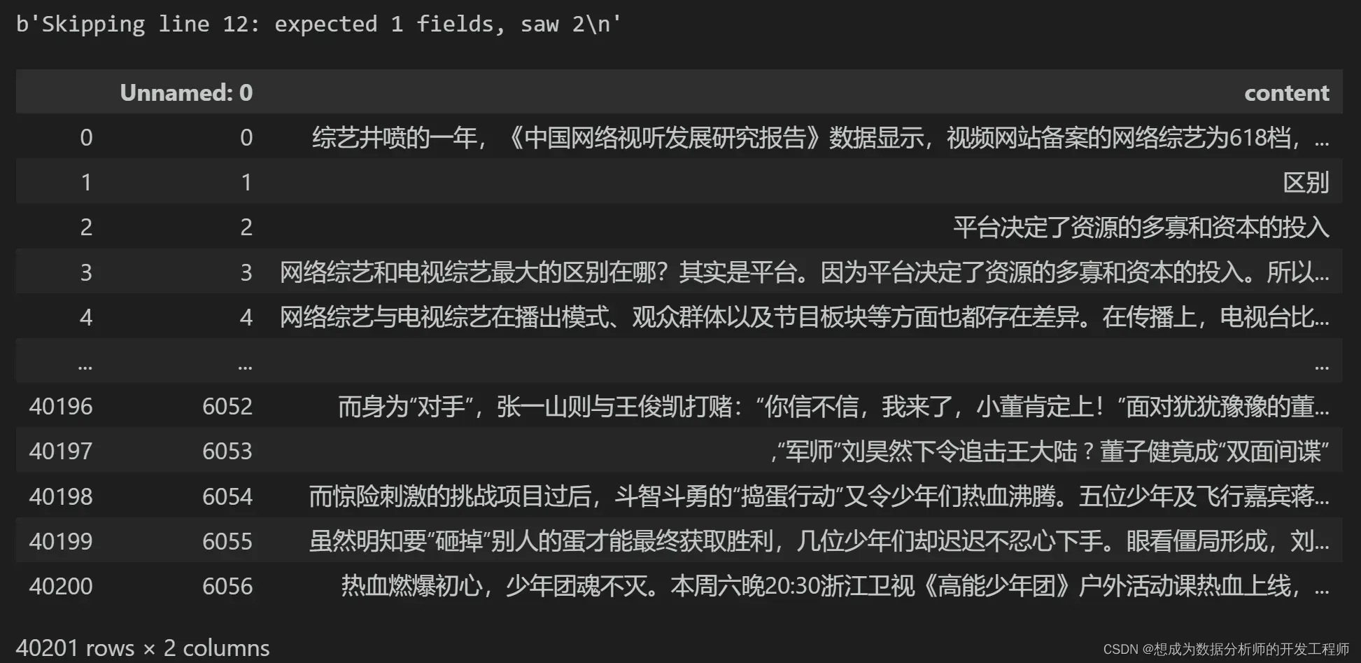
df = pd.read_csv('./data/entertainment_news.csv',encoding='gbk')
# 解决报错:ParserError: Error tokenizing data. C error: Expected 1 fields in line 12, saw 2
# 当我们使用read_csv读取txt文本文件时候,需要添加quoting=3和names指定列的参数,若还是不行则error_bad_lines=False
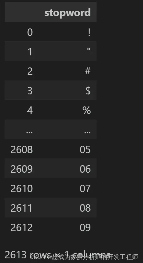
stopwords = pd.read_csv('./data/stopwords.txt',quoting=3, names=['stopword'],error_bad_lines=False)
# 2.数据查看
df
stopwords
# 2.数据预处理
# 删除空数据
df = df.dropna()
content = df.content.values.tolist()
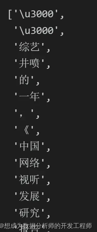
content[0]
# 测试分词
jieba.lcut(content[0])
# 测试后发现,存在一些空格、换行、标点符号等是不需要的

# 正式开始分词
segment = []
# 遍历每一行娱乐新闻数据
for line in content:
try:
segs = jieba.lcut(line) # 对每一条娱乐新闻进行分词
for seg in segs:
# 只有长度大于1的字符并且该字符不能为空格换行,这样的词语才认为是有效分词
if len(seg) > 1 and seg!='\r\n':
segment.append(seg)
except:
print(line)
continue
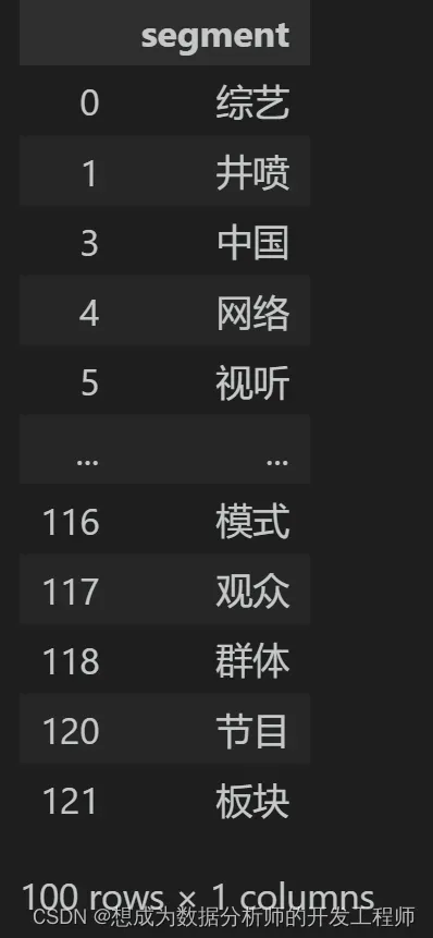
# 新建DataFrame,存储原始的分词结果
words_df = pd.DataFrame({'segment':segment})
# 去除停用词语
words_df = words_df[~words_df.segment.isin(stopwords.stopword)]
words_df.head(100)
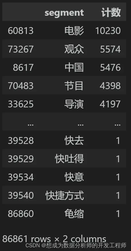
4.2 统计词频
words_stat = words_df.groupby(by='segment')['segment'].agg([('计数','count')])
words_stat = words_stat.reset_index().sort_values(by=['计数'],ascending=False)
words_stat
4.3 关键词抽取
4.3.1 基于 TF-IDF 算法的关键词抽取
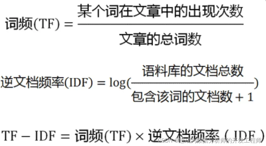
TF-IDF的思想:如果一个词或短语在一篇文章中出现的概率高,并且在其他文章中很少出现,则认为该词或短语具有很好的类别区分能力,适合用来分类
TF-IDF的作用:评估一个词语对于语料库中的某个文档的重要程度
词频:(term frequency,tf):某个词语在文档中的出现频率 逆文档频率(inverse document frequency,idf)某个词的普遍重要性的度量。由总文档数量除以包含该词的文档数量,再将得到的商取以10为底的对数 TF-IDF = TF x IDF
import jieba.analyse


jieba.analyse.extract_tags(sentence, topK=20, withWeight=False, allowPOS=())
 参数:
 - sentence 为待提取的文本
 - topK 为返回几个 TF-IDF 权重最大的关键词,默认值为 20
 - withWeight 是否一并返回关键词权重值,默认值为 False
 - allowPOS 仅包括指定词性的词,默认值为空,即不筛选
import jieba.analyse as analyse
df = pd.read_csv('data/technology_news.csv',encoding='gbk')
df = df.dropna()
# 获取每一行信息,转化为列表
lines = df.content.values.tolist()
# 使用空字符串连接列表中的每一行内容
content = "".join(lines)
# 打印前30个TF-IDF得到的关键词
print(analyse.extract_tags(content, topK=30))

4.3.2 基于 TextRank 算法的关键词抽取
jieba.analyse.textrank(sentence, topK=20, withWeight=False, allowPOS=('ns', 'n', 'vn', 'v')) 直接使用,接口相同,注意默认过滤词性
算法论文: TextRank: Bringing Order into Texts
基本思想:
- 将待抽取关键词的文本进行分词
- 以固定窗口大小(默认为5,通过span属性调整),词之间的共现关系,构建图
- 计算图中节点的PageRank
import jieba.analyse as analyse
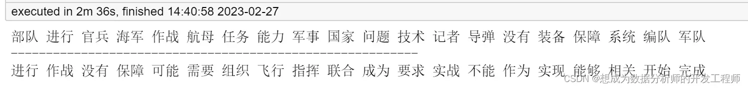
# 读取军事新闻数据
df = pd.read_csv('data/military_news.csv')
# 删除空行
df = df.dropna()
# 将新闻的每一行内容提取到列表中
lines = df.content.values.tolist()
# 将列表中的内容使用空字符串进行连接
content = "".join(lines)
# allowPOS参数可以用来限定返回的关键词次性,比如:'n'代表名称,'v'代表动词
print(" ".join(analyse.textrank(content, topK=20, allowPOS=('v','n'))))
print('----------------------------------------------------------')
print(" ".join(analyse.textrank(content, topK=20, allowPOS=('v'))))
4.4 关键词匹配——词袋模型(BOW,bag of words)
例句: Jane wants to go to Shenzhen.
Bob wants to go to Shanghai.
将所有词语装进一个袋子里,不考虑其词法和语序的问题,即每个词语都是独立的。例如上面2个例句,就可以构成一个词袋,袋子里包括Jane、wants、to、go、Shenzhen、Bob、Shanghai。假设建立一个数组(或词典)用于映射匹配
[Jane, wants, to, go, Shenzhen, Bob, Shanghai]
那么上面两个例句就可以用以下两个向量表示,对应的下标与映射数组的下标相匹配,其值为该词语出现的次数
[1,1,2,1,1,0,0]
[0,1,2,1,0,1,1]
这两个词频向量就是词袋模型,可以很明显的看到语序关系已经完全丢失
注意
在实际应用中,很多python包会分别处理每个句子,查找该句子中每个单词出现的次数,将每个句子转换为对应的向量(这种情况下,向量的长度可能不同)
import jieba
# 将数据集转换成合适的格式
df = pd.read_csv('data/technology_news.csv',encoding='gbk')
df = df.dropna()
lines = df.content.values.tolist()
# 存储每一行的分词列表
sentences = []
for line in lines:
try:
segs = jieba.lcut(line) # 对当前行分词
segs = list(filter(lambda x:len(x)>1, segs))# 过滤:只保留长度大于1的词语
segs = list(filter(lambda x:x not in stopwords, segs)) # 去除停用词
sentences.append(segs) # 将当前行分词列表添加到sentences列表中
except:
print(line)
continue
# 词袋模型处理
# gensim是应该python的自然语言处理库
from gensim import corpora
import gensim
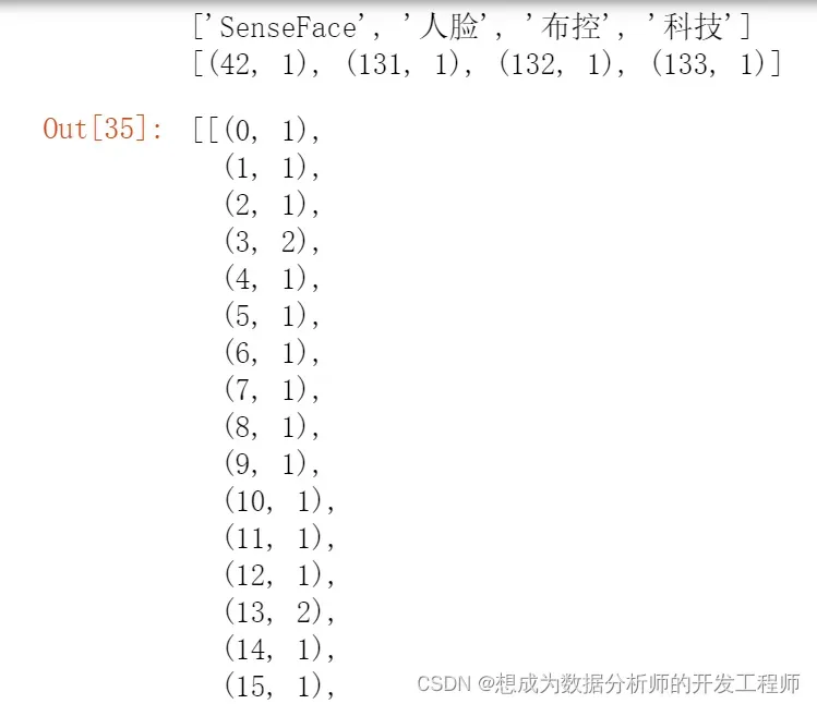
# 将sentences交给Dictionary对象
dictionary = corpora.Dictionary(sentences)
# 分别对每一行的文本分词列表转化为词袋模型
corpus = [dictionary.doc2bow(sentence) for sentence in sentences]
# 观察结果
print(sentences[3])
print(corpus[3])
corpus # (第几个词语,出现的次数)
5.绘制词云图
5.1 不使用背景图
wordcloud = WordCloud(font_path='data/simhei.ttf', background_color='white', max_font_size=80)
# 统计频率最高的1000个词语
word_frequence = {x[0]:x[1] for x in words_stat.head(1000).values}
# 对词语进行训练
wordcloud = wordcloud.fit_words(word_frequence)
# 绘制词云图
plt.imshow(wordcloud)
plt.show()

5.2 自定义背景图
当我们使用自定义背景图时,效果就是:让词云的排版样式仿照我们背景图的排版,同样的,对于颜色的使用也是根据背景图去排版
背景图

import imageio
# 设置图像大小
matplotlib.rcParams['figure.figsize'] = (15.0, 15.0)
# 读取词云背景图: 背景图的含义是根据背景图的展示布局、颜色,绘制出类似效果的词云图
bimg = imageio.imread('image/entertainment.jpeg')
# 通过WordCloud的mask参数指定词云背景图
wordcloud = WordCloud(background_color="white", mask=bimg,
                        font_path='data/simhei.ttf',max_font_size=100)
# 将词频信息转换为字典
word_frequence = {x[0]:x[1] for x in words_stat.head(1000).values}
# 学习词频信息
wordcloud = wordcloud.fit_words(word_frequence)
from wordcloud import ImageColorGenerator
# 从背景图提取颜色信息
bimgColors = ImageColorGenerator(bimg)
# 关闭坐标轴
plt.axis('off')
plt.imshow(wordcloud.recolor(color_func=bimgColors))
plt.show()

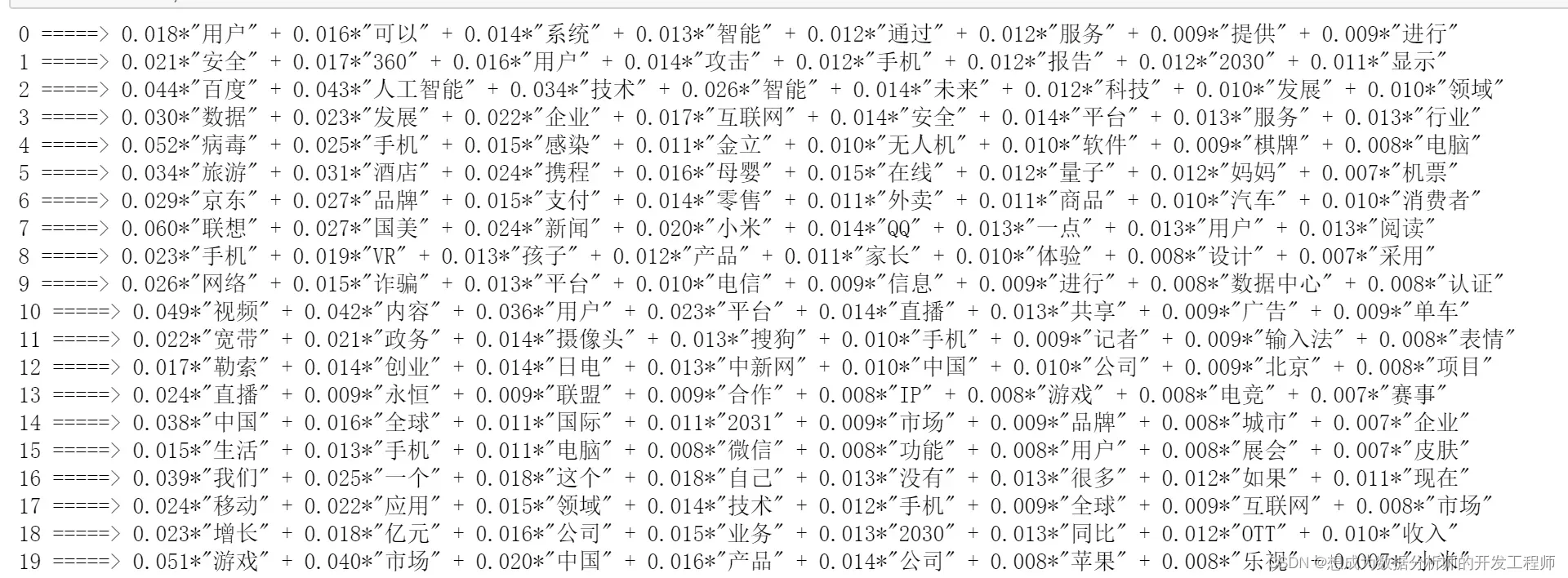
6.建模
6.1 LDA建模——文本分类主题
LDA简介
- LDA(Latent Dirichlet Allocation),也成为”隐狄利克雷分布”。 LDA 在主题模型中占有非常重要的地位,常用来文本分类。
- LDA根据一篇已有的文章,去寻找这篇文章的若干个主题,以及这些主题对应的词语
LDA建模注意事项:
用LDA主题模型建模首先要把文本内容处理成固定的格式,一个包含句子的list,list中每个元素是一句话分词后的词list。类似下面这个样子:
[[第,一,条,新闻,在,这里],[第,二,条,新闻,在,这里],[这,是,在,做, 什么],…]
# gensim是应该python自然语言处理库,能够将文档根据TF-IDF等模型转换成向量模式
from gensim import corpora, models, similarities
import gensim
# 存储每一行的分词列表 sentences [[, , ,],[, , ,],[, , ,]]
# 将sentences交给DIctionary对象
dictionary = corpora.Dictionary(sentences)
# 分别对每一行的文本分词列表转化为词袋模型(向量)
corpus = [dictionary.doc2bow(sentence) for sentence in sentences]
# 创建LdaModel对象,设置主题个数,词袋模型(向量)
# corpus:文本分词转化为词袋模型的列表;id2word:将分词列表传递给Dictionary对象;num_topics:包含的主题数量
lda = gensim.models.ldamodel.LdaModel(corpus=corpus, id2word=dictionary, num_topics=20)
# 把所有的主题都打印出来,设置要大于的主题数量,主题包含的词语数量
for topic in lda.print_topics(num_topics=20,num_words=8):
    print(topic[0],'=====>',topic[1])
7.用机器学习的方法完成中文文本分类
7.1 准备数据
import jieba
import pandas as pd
df_technology = pd.read_csv("./data/technology_news.csv", encoding='gbk')
df_technology = df_technology.dropna()

df_car = pd.read_csv("./data/car_news.csv")
df_car = df_car.dropna()

df_entertainment = pd.read_csv("./data/entertainment_news.csv", encoding='gbk')
df_entertainment = df_entertainment.dropna()

df_military = pd.read_csv("./data/military_news.csv")
df_military = df_military.dropna()

df_sports = pd.read_csv("./data/sports_news.csv")
df_sports = df_sports.dropna()

technology = df_technology.content.values.tolist()[1000:21000]
car = df_car.content.values.tolist()[1000:21000]
entertainment = df_entertainment.content.values.tolist()[:20000]
military = df_military.content.values.tolist()[:20000]
sports = df_sports.content.values.tolist()[:20000]

# 读取停用词
# stopwords=pd.read_csv("data/stopwords.txt",quoting=3,names=['stopword'])
# 解决报错:ParserError: Error tokenizing data. C error: Expected 1 fields in line 12, saw 2
# 当我们使用read_csv读取txt文本文件时候,需要添加quoting=3和names指定列的参数,若还是不行则error_bad_lines=False
stopwords = pd.read_csv('./data/stopwords.txt',quoting=3, names=['stopword'],error_bad_lines=False)
stopwords=stopwords['stopword'].values

# 去停用词
def preprocess_text(content_lines, sentences, category):
    for line in content_lines:
        try:
            segs=jieba.lcut(line)  # jieba中文分词
            segs = filter(lambda x:len(x)>1, segs) # 将文本长度大于1的留下
            segs = filter(lambda x:x not in stopwords, segs)  # 去除分词中包含停用词的分词
            # 这次也记录了每个文本的所属分类
            sentences.append((" ".join(segs), category))
        except Exception as e:
            print(line)
            continue

#生成训练数据
sentences = []
preprocess_text(technology, sentences, 'technology')
preprocess_text(car, sentences, 'car')
preprocess_text(entertainment, sentences, 'entertainment')
preprocess_text(military, sentences, 'military')
preprocess_text(sports, sentences, 'sports')

# 打乱一下顺序,生成更可靠的训练集
import random
random.shuffle(sentences)
# 观察一下
for sentence in sentences[:10]:
    print(sentence[0], sentence[1])
# 为了一会儿检测一下分类器效果怎么样,需要一份测试集。
# 所以把原数据集分成训练集的测试集,用sklearn自带的分割函数
from sklearn.model_selection import train_test_split
x, y = zip(*sentences)
x_train, x_test, y_train, y_test = train_test_split(x, y, random_state=1234)
len(x_train)
7.2 朴素贝叶斯使用简介
7.2.1 简介
- 朴素贝叶斯(naïve Bayes)法是基于贝叶斯定理与特征条件独立假设的分类方法。
- “朴素”的含义:样本的各特征之间相互独立。
- 算法原理:对于待分类样本,计算在此待分类样本出现的条件下各个类别出现的概率,哪个最大,就认为此样本属于哪个类别
7.2.2 对文本抽取词袋模型特征简介
对于文本来说,预处理时需要把文本转换为数字类型
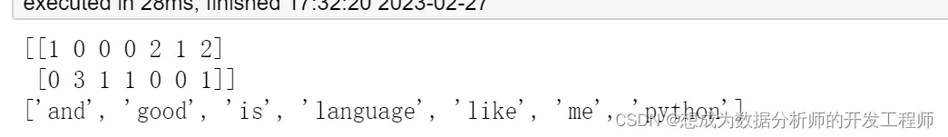
CountVectorizer
**作用:**用来统计样本中特征词出现的个数,将单词作为特征(特征词)
例子:
data = ["i like python,and python like me",
        "python is a good good good language"]
from sklearn.feature_extraction.text import CountVectorizer
cv = CountVectorizer()
transform_data = cv.fit_transform(data)  # 拟合+转换文本
print(transform_data.toarray())
print(cv.get_feature_names())  # 提取的特征词
7.2.3 使用MultinomialNB实现朴素贝叶斯
from sklearn.naive_bayes import MultinomialNB
classifier = MultinomialNB()
classifier.fit(训练样本集特征,训练样本集标签)  # 拟合训练
# 在测试集上测试准确率
classifier.score(测试样本集特征,测试样本集标签)
7.3 模型训练
# 1.对文本抽取词袋模型特征
from sklearn.feature_extraction.text import CountVectorizer
# 设置最大的特征数量为4000
vec = CountVectorizer(max_features=4000)
vec.fit(x_train) # 拟合训练
# 2.使用朴素贝叶斯进行文本分类
from sklearn.naive_bayes import MultinomialNB
classifier = MultinomialNB()
# 拟合进行分类训练,注意:传递的样本特征一定要先转化为词袋模型(数字向量)
classifier.fit(vec.transform(x_train),y_train)
# 3.评价分类结果
classifier.score(vec.transform(x_test),y_test)
0.8442394629891776
7.4 自定义文本分类器(模型)完成中文文本分类
本质上还是调用朴素贝叶斯算法,只是单独制作成了一个类
import re
from sklearn.feature_extraction.text import CountVectorizer
from sklearn.model_selection import train_test_split
from sklearn.naive_bayes import MultinomialNB

class TextClassifier:
    def __init__(self, classifier=MultinomialNB()):
        # 自定义初始化,默认使用分类器时朴素贝叶斯
        self.classifier = classifier # 分类器对象
        self.vectorizer = CountVectorizer(max_features=4000) # 词袋实现对象

    # 词袋实现,文本转换成数字向量
    def features(self, X):
        return self.vectorizer.transform(X)

    # 训练模型
    def fit(self, X, y):
        # 词袋拟合模型
        self.vectorizer.fit(X)
        # 分类训练(特征转换为数字向量)
        self.classifier.fit(self.features(X),y)

    # 对某个文本预测
    def predict(self, x):
        return self.classifier.predict(self.features([x]))

    # 准确率
    def score(self,X,y):
        return self.classifier.score(self.features(X),y)
# 实例化对象
text_classifier = TextClassifier()
# 拟合训练
text_classifier.fit(x_train,y_train)
# 在测试集上查看准确率
print(text_classifier.score(x_test,y_test))
# 预测
print(text_classifier.predict("多年 百变 歌喉 海燕 这位 酷爱 邓丽君 歌曲 并视 歌唱 生命 歌者"))
8.用深度学习的方法完成中文文本分类
8.1 CNN做文本分类
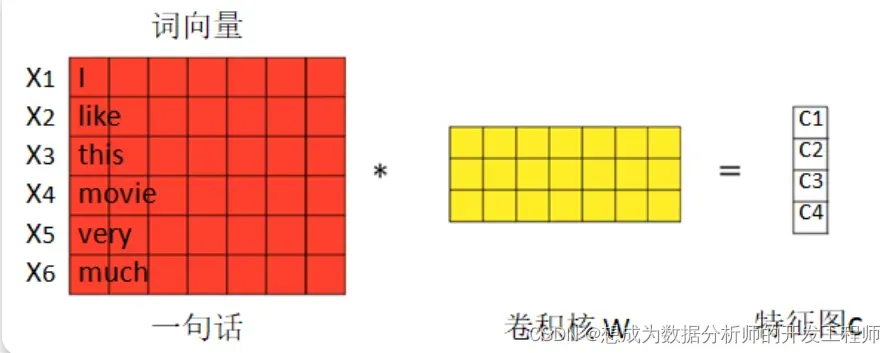
卷积神经网络(Convolutional Neural Network,CNN)也适合做的是文本分类,由于卷积和池化会丢失句子局部字词的排列关系,所以纯cnn不太适合序列标注和命名实体识别之类的任务。
nlp任务的输入都不再是图片像素,而是以矩阵表示的句子或者文档。矩阵的每一行对应一个单词或者字符。也即每行代表一个词向量,通常是像 word2vec 或 GloVe 词向量。在图像问题中,卷积核滑过的是图像的一“块”区域,但在自然语言领域里我们一般用卷积核滑过矩阵的一“行”(单词)。
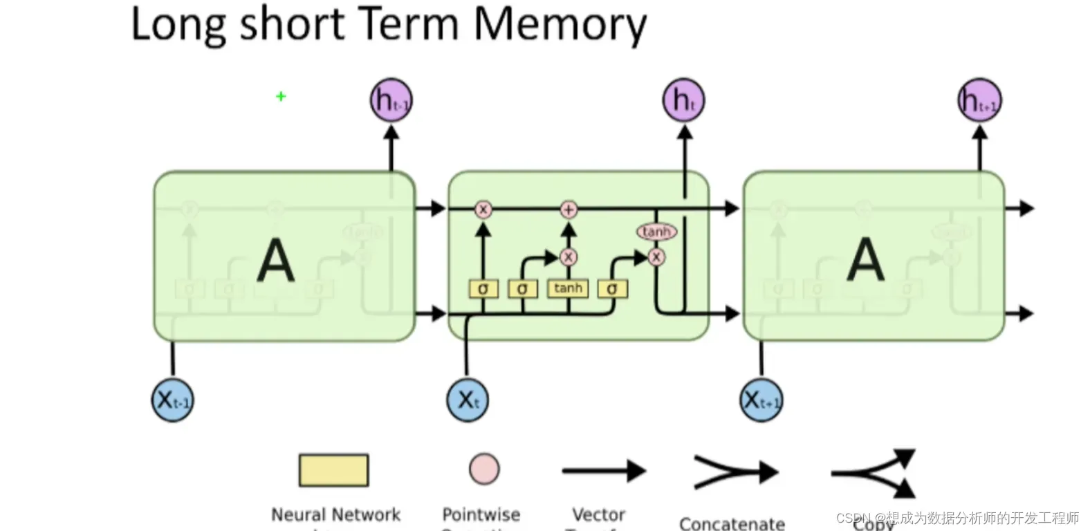
8.2 LSTM文本分类
能捕捉时序信息的长短时记忆神经网络LSTM,毕竟,对于长文的信息捕捉,凭借自带的Memory属性,它还是有比较强的能力的
"""
使用RNN完成文本分类
"""

from __future__ import absolute_import
from __future__ import division
from __future__ import print_function

import argparse
import sys

import numpy as np
import pandas
from sklearn import metrics
import tensorflow as tf
from tensorflow.contrib.layers.python.layers import encoders

learn = tf.contrib.learn

FLAGS = None

MAX_DOCUMENT_LENGTH = 15
MIN_WORD_FREQUENCE = 1
EMBEDDING_SIZE = 50
global n_words
# 处理词汇
vocab_processor = learn.preprocessing.VocabularyProcessor(MAX_DOCUMENT_LENGTH, min_frequency=MIN_WORD_FREQUENCE)
x_train = np.array(list(vocab_processor.fit_transform(train_data)))
x_test = np.array(list(vocab_processor.transform(test_data)))
n_words = len(vocab_processor.vocabulary_)
print('Total words: %d' % n_words)

def bag_of_words_model(features, target):
    """先转成词袋模型"""
    target = tf.one_hot(target, 15, 1, 0)
    features = encoders.bow_encoder(
            features, vocab_size=n_words, embed_dim=EMBEDDING_SIZE)
    logits = tf.contrib.layers.fully_connected(features, 15, activation_fn=None)
    loss = tf.contrib.losses.softmax_cross_entropy(logits, target)
    train_op = tf.contrib.layers.optimize_loss(
            loss,
            tf.contrib.framework.get_global_step(),
            optimizer='Adam',
            learning_rate=0.01)
    return ({
            'class': tf.argmax(logits, 1),
            'prob': tf.nn.softmax(logits)
    }, loss, train_op)


model_fn = bag_of_words_model
classifier = learn.SKCompat(learn.Estimator(model_fn=model_fn))

# Train and predict
classifier.fit(x_train, y_train, steps=1000)
y_predicted = classifier.predict(x_test)['class']
score = metrics.accuracy_score(y_test, y_predicted)
print('Accuracy: {0:f}'.format(score))
def rnn_model(features, target):
    """用RNN模型(这里用的是GRU)完成文本分类"""
    # Convert indexes of words into embeddings.
    # This creates embeddings matrix of [n_words, EMBEDDING_SIZE] and then
    # maps word indexes of the sequence into [batch_size, sequence_length,
    # EMBEDDING_SIZE].
    word_vectors = tf.contrib.layers.embed_sequence(
            features, vocab_size=n_words, embed_dim=EMBEDDING_SIZE, scope='words')

    # Split into list of embedding per word, while removing doc length dim.
    # word_list results to be a list of tensors [batch_size, EMBEDDING_SIZE].
    word_list = tf.unstack(word_vectors, axis=1)

    # Create a Gated Recurrent Unit cell with hidden size of EMBEDDING_SIZE.
    cell = tf.contrib.rnn.GRUCell(EMBEDDING_SIZE)

    # Create an unrolled Recurrent Neural Networks to length of
    # MAX_DOCUMENT_LENGTH and passes word_list as inputs for each unit.
    _, encoding = tf.contrib.rnn.static_rnn(cell, word_list, dtype=tf.float32)

    # Given encoding of RNN, take encoding of last step (e.g hidden size of the
    # neural network of last step) and pass it as features for logistic
    # regression over output classes.
    target = tf.one_hot(target, 15, 1, 0)
    logits = tf.contrib.layers.fully_connected(encoding, 15, activation_fn=None)
    loss = tf.contrib.losses.softmax_cross_entropy(logits, target)

    # Create a training op.
    train_op = tf.contrib.layers.optimize_loss(
            loss,
            tf.contrib.framework.get_global_step(),
            optimizer='Adam',
            learning_rate=0.01)

    return ({
            'class': tf.argmax(logits, 1),
            'prob': tf.nn.softmax(logits)
    }, loss, train_op)

model_fn = rnn_model
classifier = learn.SKCompat(learn.Estimator(model_fn=model_fn))

# Train and predict
classifier.fit(x_train, y_train, steps=1000)
y_predicted = classifier.predict(x_test)['class']
score = metrics.accuracy_score(y_test, y_predicted)
print('Accuracy: {0:f}'.format(score))
版权声明:本文为博主作者:想成为数据分析师的开发工程师原创文章,版权归属原作者,如果侵权,请联系我们删除!
原文链接:https://blog.csdn.net/m0_63953077/article/details/129225150