一、简介
-
pandas是一个强大的Python数据分析的工具包,是基于NumPy构建
-
pandas的主要功能:
- 具备对其功能的数据结构DataFrame、Series
- 集成时间序列功能
- 提供丰富的教学运算和操作
- 灵活处理缺失数据
-
安装:pip3 install pandas
二、Series
1、简介
Series是一种类似于一维数组的对象,由一组数据和一组与之相关的数据标签(索引)组成
Series比较像列表(数组)和字典的结合体

Series支持array的特性(下标):
  从ndarray创建Series:Series(arr)
  与标量运算:sr*2
  两个Series运算:sr1+sr2
  索引:sr[0],sr[[1, 2, 3]]
  切片:sr[0:2]
  通用函数:np.abs(sr)
  布尔值过滤:sr[sr>0]

Series支持字典的特性(标签):
  从字典创建Series:Series(dic)
  in运算:'a' in sr
  键索引:sr['a'],sr[['a', 'b', 'd']]
2、初体验
import pandas as pd
import numpy as np

print(pd.Series([2, 3, 4]))
print('-------------------')
print(pd.Series([2, 3, 4], index=['a', 'b', 'c']))
print('-------------------')
print(pd.Series(np.arange(3)))
结果:
0    2
1    3
2    4
dtype: int64
-------------------
a    2
b    3
c    4
dtype: int64
-------------------
0    0
1    1
2    2
dtype: int64
3、series索引
import pandas as pd
import numpy as np

sr = pd.Series(np.arange(4))
sr1 = sr[2:].copy()
print(sr1)
print('-----------------------')
print(sr1.loc[3], sr1.iloc[0])
结果:
2    2
3    3
dtype: int64
-----------------------
3 2
4、series数据对齐
import pandas as pd

sr1 = pd.Series([1, 2, 3], index=['c', 'a', 'b'])
sr2 = pd.Series([4, 5, 6], index=['b', 'c', 'a'])
sr3 = pd.Series([4, 5, 6, 7], index=['b', 'c', 'a', 'd'])
print(sr1 + sr2)
print('------------')
print(sr1 + sr3)
print('------------')
print(sr1.add(sr3, fill_value=0))
结果:
a    8
b    7
c    6
dtype: int64
------------
a    8.0
b    7.0
c    6.0
d    NaN
dtype: float64
------------
a    8.0
b    7.0
c    6.0
d    7.0
dtype: float64
5、series缺失值处理
import pandas as pd

sr1 = pd.Series([1, 2, 3], index=['c', 'a', 'b'])
sr2 = pd.Series([4, 5, 6], index=['b', 'c', 'd'])
sr = sr1 + sr2
print(sr)
print('-------------------')
print(sr.isnull())
print('-------------------')
print(sr.notnull())
print('-------处理缺失值-------')
print(sr[sr.notnull()])
print('-------处理缺失值-------')
print(sr.dropna())
print('-------------------')
print(sr.fillna(0))
print('-------------------')
print(sr.fillna(sr.mean()))
结果:
a    NaN
b    7.0
c    6.0
d    NaN
dtype: float64
-------------------
a     True
b    False
c    False
d     True
dtype: bool
-------------------
a    False
b     True
c     True
d    False
dtype: bool
-------处理缺失值-------
b    7.0
c    6.0
dtype: float64
-------处理缺失值-------
b    7.0
c    6.0
dtype: float64
-------------------
a    0.0
b    7.0
c    6.0
d    0.0
dtype: float64
-------------------
a    6.5
b    7.0
c    6.0
d    6.5
dtype: float64
三、DataFrame
DataFrame是一个表格型的数据结构,含有一组有序的列。DataFrame可以被看做是由Series组成的字典
1、DataFrame创建
import pandas as pd
df = pd.DataFrame({'one': [1, 2, 3], 'tow': [4, 5, 6]}, index=['a', 'b', 'c'])
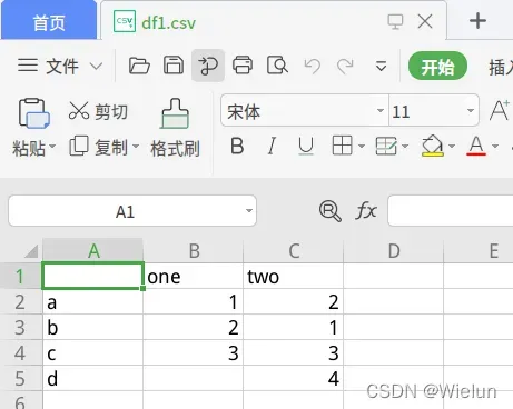
df1 = pd.DataFrame(
{'one': pd.Series([1, 2, 3], index=['a', 'b', 'c']), 'two': pd.Series([1, 2, 3, 4], index=['b', 'a', 'c', 'd'])})
print(df)
print('--------------')
print(df1)
df1.to_csv('df1.csv')
print('--------------')
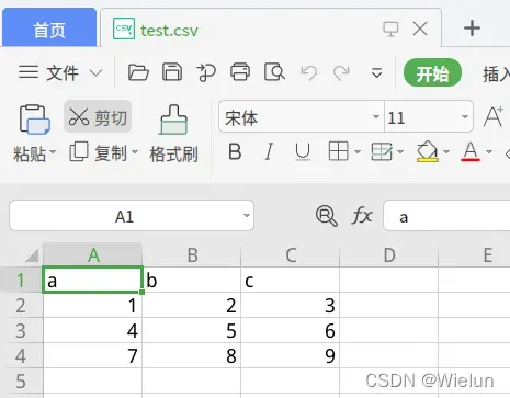
print(pd.read_csv('test.csv'))
结果:
   one  tow
a    1    4
b    2    5
c    3    6
--------------
   one  two
a  1.0    2
b  2.0    1
c  3.0    3
d  NaN    4
--------------
   a  b  c
0  1  2  3
1  4  5  6
2  7  8  9
2、DataFrame常用属性
index         获取索引
T             转置
columns       获取列索引
values        获取值数组
describe()    获取快速统计
import pandas as pd

df = pd.DataFrame({'one': [1, 2, 3], 'tow': [4, 5, 6]}, index=['a', 'b', 'c'])
print(df)
print('---------------')
print(df.index)
print('---------------')
print(df.values)
print('---------------')
print(df.T)
print('---------------')
print(df.columns)
print('---------------')
print(df.describe())
结果:
   one  tow
a    1    4
b    2    5
c    3    6
---------------
Index(['a', 'b', 'c'], dtype='object')
---------------
[[1 4]
 [2 5]
 [3 6]]
---------------
     a  b  c
one  1  2  3
tow  4  5  6
---------------
Index(['one', 'tow'], dtype='object')
---------------
       one  tow
count  3.0  3.0
mean   2.0  5.0
std    1.0  1.0
min    1.0  4.0
25%    1.5  4.5
50%    2.0  5.0
75%    2.5  5.5
max    3.0  6.0
3、DataFrame索引和切片
- DataFrame是一个二维数组类型,所以有行索引和列索引
- DataFrame同样可以通过标签和位置两种方法进行索引和切片
- loc属性和iloc属性
- 使用方法:逗号隔开,前面是行索引,后面是列索引
- 行/列索引部分可以是常规索引、切片、布尔值索引任意搭配
import pandas as pd

df = pd.DataFrame({'one': [1, 2, 3], 'two': [4, 5, 6]}, index=['a', 'b', 'c'])
print(df)
print('---------------')
print(df.loc['b', 'one'])
print('---------------')
print(df.loc['a', :])
结果:
   one  two
a    1    4
b    2    5
c    3    6
---------------
2
one    1
tow    4
Name: a, dtype: int64
4、DataFrame数据对齐与缺失数据处理
- DataFrame对象在运算时,同样会进行数据对齐,其行索引和列索引分别对齐
- DataFrame处理缺失数据的相关的方法:
- dropna(axis=0,where=‘any’,…)
- fillna()
- isnull()
- notnull()
import pandas as pd
import numpy as np

df = pd.DataFrame({'one': [1, 2, 3], 'two': [4, 5, 6]}, index=['a', 'b', 'c'])
df1 = pd.DataFrame({'one': [1, 2, 3, 4], 'two': [5, 6, 7, 8]}, index=['a', 'b', 'c', 'd'])
df.loc['c', 'two'] = np.nan
df2 = df + df1
print(df2)
print('-----------------')
print(df2.fillna(0))
print('-----------------')
print(df2.dropna())
print('-----------------')
print(df2.dropna(how='all'))
print('-----------------')
print(df2.dropna(how='any'))
print('-----------------')
print(df2.loc['c', 'one'])
print('-----------------')
print(df)
print(df.dropna(axis=0))  # 行
print(df.dropna(axis=1))  # 列
结果:
   one   two
a  2.0   9.0
b  4.0  11.0
c  6.0   NaN
d  NaN   NaN
-----------------
   one   two
a  2.0   9.0
b  4.0  11.0
c  6.0   0.0
d  0.0   0.0
-----------------
   one   two
a  2.0   9.0
b  4.0  11.0
-----------------
   one   two
a  2.0   9.0
b  4.0  11.0
c  6.0   NaN
-----------------
   one   two
a  2.0   9.0
b  4.0  11.0
-----------------
6.0
-----------------
   one  two
a    1  4.0
b    2  5.0
c    3  NaN
   one
a    1
b    2
c    3
   one  two
a    1  4.0
b    2  5.0
四、pandas常用函数
mean(axis=0,skipna=Faluse)          对列(行)求平均值
sum(axis=1)                         对列(行)求和
sort_index(axis, ..., ascending)    对列(行)索引排序
sort_values(by, axis, ascending)    按某一列(行)的值排序
import pandas as pd
import numpy as np

df = pd.DataFrame({'one': [2, 1, 3], 'two': [5, 4, 6]}, index=['a', 'b', 'c'])
df.loc['c', 'two'] = np.nan
print(df)
print('--------------------')
print(df.mean())
print('--------------------')
print(df.mean(axis=1))
print('--------------------')
print(df.sum(axis=1))
print('--------------------')
print(df.sort_values(by='one', ascending=False))
print('--------------------')
print(df.sort_index(ascending=False, axis=1))
结果:
   one  two
a    2  5.0
b    1  4.0
c    3  NaN
--------------------
one    2.0
two    4.5
dtype: float64
--------------------
a    3.5
b    2.5
c    3.0
dtype: float64
--------------------
a    7.0
b    5.0
c    3.0
dtype: float64
--------------------
   one  two
c    3  NaN
a    2  5.0
b    1  4.0
--------------------
   two  one
a  5.0    2
b  4.0    1
c  NaN    3
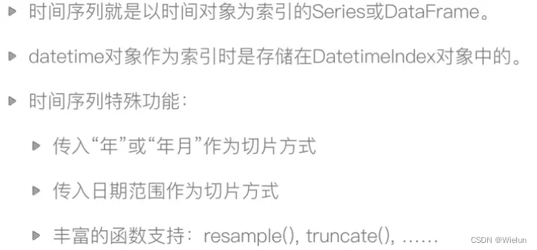
五、pandas时间对象
1、时间处理对象
产生时间对象数组:date_range
	start       开始时间
	end         结束时间
    periods     时间长度
    freq        时间频率,默认为'D',可以H(our),W(eek),B(usiness),S(emi-)M(onth),(min)T(es),S(encond),A(year),...
import pandas as pd
import datetime, dateutil

x = dateutil.parser.parse('02/03/2001')
print(x, type(x))
print(pd.date_range('2022-1-1', '2022-2-1'))
print(pd.date_range('2022-1-1', periods=10, freq='H'))
结果:
2001-02-03 00:00:00 <class 'datetime.datetime'>
DatetimeIndex(['2022-01-01', '2022-01-02', '2022-01-03', '2022-01-04',
               '2022-01-05', '2022-01-06', '2022-01-07', '2022-01-08',
               '2022-01-09', '2022-01-10', '2022-01-11', '2022-01-12',
               '2022-01-13', '2022-01-14', '2022-01-15', '2022-01-16',
               '2022-01-17', '2022-01-18', '2022-01-19', '2022-01-20',
               '2022-01-21', '2022-01-22', '2022-01-23', '2022-01-24',
               '2022-01-25', '2022-01-26', '2022-01-27', '2022-01-28',
               '2022-01-29', '2022-01-30', '2022-01-31', '2022-02-01'],
              dtype='datetime64[ns]', freq='D')
DatetimeIndex(['2022-01-01 00:00:00', '2022-01-01 01:00:00',
               '2022-01-01 02:00:00', '2022-01-01 03:00:00',
               '2022-01-01 04:00:00', '2022-01-01 05:00:00',
               '2022-01-01 06:00:00', '2022-01-01 07:00:00',
               '2022-01-01 08:00:00', '2022-01-01 09:00:00'],
              dtype='datetime64[ns]', freq='H')
2、时间序列
import numpy as np
import pandas as pd

sr = pd.Series(np.arange(50), index=pd.date_range('2021-12-25', periods=50))

print(sr)
print('-----------------------------')
print(sr['2022-02'])
print('-----------------------------')
print(sr['2021'])
print('-----------------------------')
print(sr['2021-12-25':'2021-12-27'])
print('-----------------------------')
print(sr.resample('W').sum()) # 周求和,月:M
结果:
2021-12-25     0
2021-12-26     1
2021-12-27     2
2021-12-28     3
2021-12-29     4
2021-12-30     5
2021-12-31     6
2022-01-01     7
2022-01-02     8
2022-01-03     9
2022-01-04    10
2022-01-05    11
2022-01-06    12
2022-01-07    13
2022-01-08    14
2022-01-09    15
2022-01-10    16
2022-01-11    17
2022-01-12    18
2022-01-13    19
2022-01-14    20
2022-01-15    21
2022-01-16    22
2022-01-17    23
2022-01-18    24
2022-01-19    25
2022-01-20    26
2022-01-21    27
2022-01-22    28
2022-01-23    29
2022-01-24    30
2022-01-25    31
2022-01-26    32
2022-01-27    33
2022-01-28    34
2022-01-29    35
2022-01-30    36
2022-01-31    37
2022-02-01    38
2022-02-02    39
2022-02-03    40
2022-02-04    41
2022-02-05    42
2022-02-06    43
2022-02-07    44
2022-02-08    45
2022-02-09    46
2022-02-10    47
2022-02-11    48
2022-02-12    49
Freq: D, dtype: int64
-----------------------------
2022-02-01    38
2022-02-02    39
2022-02-03    40
2022-02-04    41
2022-02-05    42
2022-02-06    43
2022-02-07    44
2022-02-08    45
2022-02-09    46
2022-02-10    47
2022-02-11    48
2022-02-12    49
Freq: D, dtype: int64
-----------------------------
2021-12-25    0
2021-12-26    1
2021-12-27    2
2021-12-28    3
2021-12-29    4
2021-12-30    5
2021-12-31    6
Freq: D, dtype: int64
-----------------------------
2021-12-25    0
2021-12-26    1
2021-12-27    2
Freq: D, dtype: int64
-----------------------------
2021-12-26      1
2022-01-02     35
2022-01-09     84
2022-01-16    133
2022-01-23    182
2022-01-30    231
2022-02-06    280
2022-02-13    279
Freq: W-SUN, dtype: int64
六、pandas文件处理
1、简介
- 数据文件常用格式:csv
- pandas读取文件:从文件名、URL、文件对象中加载数据
- read_csv:默认分隔符为逗号
- read_table:默认分隔符为制表符
read_csv、read_table函数主要参数:
    sep             指定分隔符,可用正则表达式入'\s+'
    header=None     指定文件无列名
    name            指定列名
    index_col       指定某列作为索引
    skip_row        指定跳过某些行
    na_values       指定某些字符串表示缺失值
    parse_dates     指定某些列是否被解析为日期,类型为布尔值或列表
2、read_csv函数
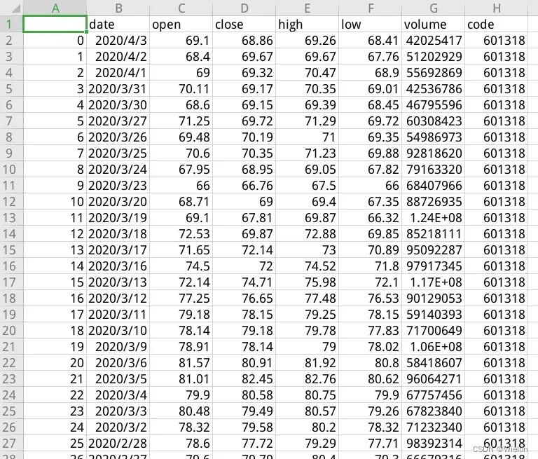
import pandas as pd

# parse_dates:解析为时间对象,默认为str
df = pd.read_csv('601318.csv', index_col='date', parse_dates=True)
print(df)
df = pd.read_csv('601318.csv', header=None, names=list('abcdefg'))
print(df)
结果:
            Unnamed: 0   open  close   high    low    volume    code
date
2020-04-03           0  69.10  68.86  69.26  68.41  42025417  601318
2020-04-02           1  68.40  69.67  69.67  67.76  51202929  601318
2020-04-01           2  69.00  69.32  70.47  68.90  55692869  601318
2020-03-31           3  70.11  69.17  70.35  69.01  42536786  601318
2020-03-30           4  68.60  69.15  69.39  68.45  46795596  601318
...                ...    ...    ...    ...    ...       ...     ...
2019-01-11         297  58.00  58.07  58.29  57.50  45756973  601318
2019-01-10         298  56.87  57.50  57.82  56.55  67328223  601318
2019-01-09         299  56.20  56.95  57.60  55.96  81914613  601318
2019-01-08         300  56.05  55.80  56.09  55.20  55992092  601318
2019-01-07         301  57.09  56.30  57.17  55.90  76593007  601318

[302 rows x 7 columns]
               a      b      c      d      e         f       g
NaN         date   open  close   high    low    volume    code
0.0     2020/4/3   69.1  68.86  69.26  68.41  42025417  601318
1.0     2020/4/2   68.4  69.67  69.67  67.76  51202929  601318
2.0     2020/4/1     69  69.32  70.47   68.9  55692869  601318
3.0    2020/3/31  70.11  69.17  70.35  69.01  42536786  601318
...          ...    ...    ...    ...    ...       ...     ...
297.0  2019/1/11     58  58.07  58.29   57.5  45756973  601318
298.0  2019/1/10  56.87   57.5  57.82  56.55  67328223  601318
299.0   2019/1/9   56.2  56.95   57.6  55.96  81914613  601318
300.0   2019/1/8  56.05   55.8  56.09   55.2  55992092  601318
301.0   2019/1/7  57.09   56.3  57.17   55.9  76593007  601318
3、to_csv函数
主要参数:
    sep             指定文件分隔符
    na_rep          指定缺失值转换的字符串,默认为空字符串
    header=False    不输出列名一行
    index=False     不输出行索引一列
    cols            指定输出的列,传入列表
七、Matplotlib使用
1、简介
- Matplotlib是一个强大的Python绘图和数据可视化的工具包
- 安装方法:pip install matplotlib
plot函数:绘制折线图
  线型linestyle(-,-.,--,..)
  点型marker(v,^,s,*,H,+,x,D,o,...)
  颜色color(b,g,r,y,k,w,...)
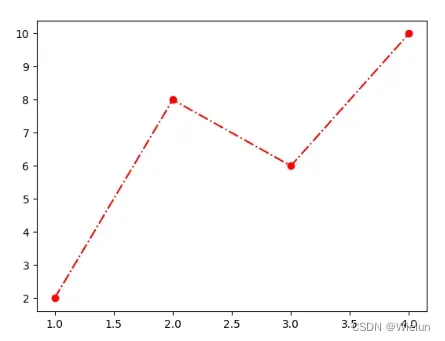
2、初体验
import matplotlib.pyplot as plt

plt.plot([1, 2, 3, 4], [2, 8, 6, 10], "o-.", color='red')  # 折线图
plt.show()
结果:
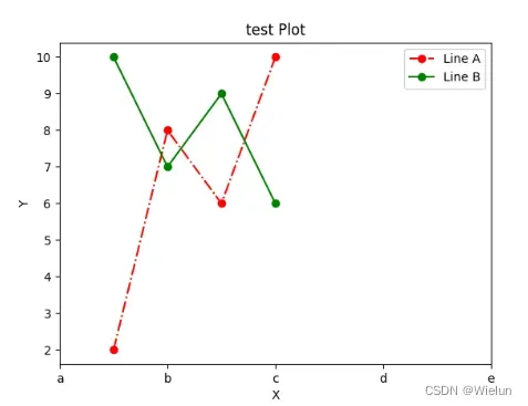
3、plot函数周边
图像标注:
    设置图像标题:plt.title()    设置y轴范围:plt.ylim()
    设置x轴名称:plt.xlabel()    设置x轴刻度:plt.xticks()
    设置y轴名称:plt.ylabel()    设置y轴刻度:plt.yticks()
    设置x轴范围:plt.xlim()      设置曲线图例:plt.legend()
import matplotlib.pyplot as plt
import numpy as np

plt.plot([1, 2, 3, 4], [2, 8, 6, 10], "o-.", color='red', label='Line A')  # 折线图
plt.plot([1, 2, 3, 4], [10, 7, 9, 6], color='green', marker='o', label='Line B')
plt.title('test Plot')
plt.xlabel('X')
plt.ylabel('Y')
plt.xticks(np.arange(0, 10, 2), ['a', 'b', 'c', 'd', 'e'])
plt.legend()
plt.show()
结果:
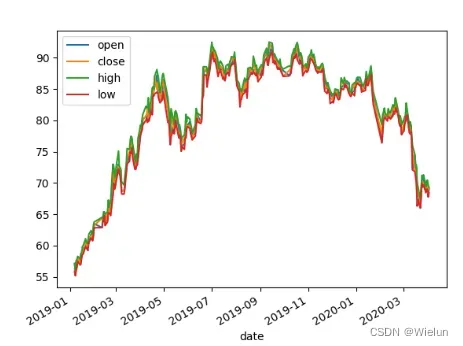
4、pandas与Matplotlib
使用上面的csv文件
(1)画股票图像
import matplotlib.pyplot as plt
import pandas as pd

df = pd.read_csv('601318.csv',parse_dates=['date'], index_col='date')[['open','close','high','low']]
df.plot()
plt.show()
结果:
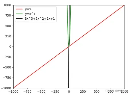
(2)案例
import matplotlib.pyplot as plt
import numpy as np

x = np.linspace(-1000, 1000, 10000)
y1 = x
y2 = x * x
y3 = 3 * x ** 3 + 5 * x ** 2 + 2 * x + 1
plt.plot(x, y1, color='red', label='y=x')
plt.plot(x, y2, color='green', label='y=x^x')
plt.plot(x, y3, color='black', label='3x^3+5x^2+2x+1')
plt.xlim(-1000, 1000)
plt.ylim(-1000, 1000)
plt.legend()
plt.show()
结果:
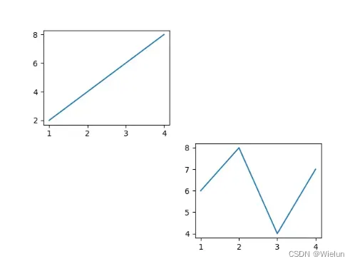
5、Matplotlib画布与子图
画布:figure
    fig = plt.figure()
图:subplot
    ax1 = fig.add_subplot(2,2,1)
调节子图间距:
    subplots_adjust(left, bottom, right, top, wspace, hspace)
import matplotlib.pyplot as plt

fig = plt.figure()
ax1 = fig.add_subplot(2, 2, 1)  # 两行两列,占第一个位置
ax1.plot([1, 2, 3, 4], [2, 4, 6, 8])

ax2 = fig.add_subplot(2, 2, 4)
ax2.plot([1, 2, 3, 4], [6, 8, 4, 7])

plt.show()
结果:
6、Matplotlib柱状图和饼图
plt.plot(x,y,fmt,...)                 坐标图
plt.boxplot(data,notch,position)      箱型图
plt.bar(left,height,width,bottom)     条形图
plt.barh(width,bottom,left,height)    横向条形图
plt.polar(theta, r)                   极坐标图
plt.pie(data, explode)                饼图
plt.psd(x,NFFT=256,pad_to,Fs)         功率谱密度图
plt.specgram(x,NFFT=256,pad_to,F)     谱图
plt.cohere(x,y,NFFT=256,Fs)           X-Y相关性函数
plt.scatter(x,y)                      散点图
plt.step(x,y,where)                   步阶图
plt.hist(x,bins,normed)               直方图
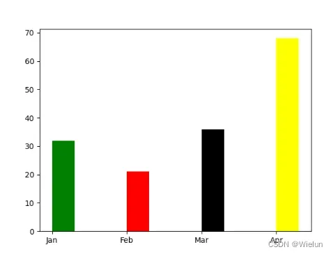
(1)bar案例
import matplotlib.pyplot as plt
import numpy as np

data = [32, 21, 36, 68]
label = ['Jan', 'Feb', 'Mar', 'Apr']
plt.bar(np.arange(len(data)), data, color=['green', 'red', 'black', 'yellow'], width=0.3, align='edge')
plt.xticks(np.arange(len(data)), labels=label)
# plt.bar([1, 2, 3, 4], [6, 8, 4, 7])
plt.show()
结果:
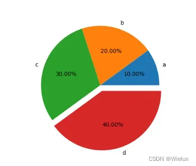
(2)pie案例
import matplotlib.pyplot as plt

plt.pie([10, 20, 30, 40], labels=['a', 'b', 'c', 'd'], autopct="%.2f%%", explode=[0, 0, 0, 0.1])
plt.show()
结果:
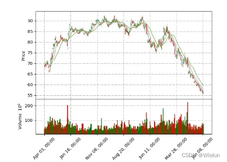
7、Matplotlib绘制K线图
安装:pip3 install mplfinance
import matplotlib.pyplot as plt
import pandas as pd
import mplfinance as mpf
from matplotlib.dates import date2num

df = pd.read_csv('601318.csv', index_col='date', parse_dates=True)
df['time'] = date2num(df.index.to_pydatetime())
print(df)
mycolor = mpf.make_marketcolors(up="red", down="green", edge="i", wick="i", volume="in")
mystyle = mpf.make_mpf_style(marketcolors=mycolor, gridaxis="both", gridstyle="-.")
mpf.plot(df, type="candle", mav=(5, 10, 20), style=mystyle, volume=True, show_nontrading=False)
plt.show()
结果:
            Unnamed: 0   open  close   high    low    volume    code     time
date
2020-04-03           0  69.10  68.86  69.26  68.41  42025417  601318  18355.0
2020-04-02           1  68.40  69.67  69.67  67.76  51202929  601318  18354.0
2020-04-01           2  69.00  69.32  70.47  68.90  55692869  601318  18353.0
2020-03-31           3  70.11  69.17  70.35  69.01  42536786  601318  18352.0
2020-03-30           4  68.60  69.15  69.39  68.45  46795596  601318  18351.0
...                ...    ...    ...    ...    ...       ...     ...      ...
2019-01-11         297  58.00  58.07  58.29  57.50  45756973  601318  17907.0
2019-01-10         298  56.87  57.50  57.82  56.55  67328223  601318  17906.0
2019-01-09         299  56.20  56.95  57.60  55.96  81914613  601318  17905.0
2019-01-08         300  56.05  55.80  56.09  55.20  55992092  601318  17904.0
2019-01-07         301  57.09  56.30  57.17  55.90  76593007  601318  17903.0
文章出处登录后可见!
已经登录?立即刷新