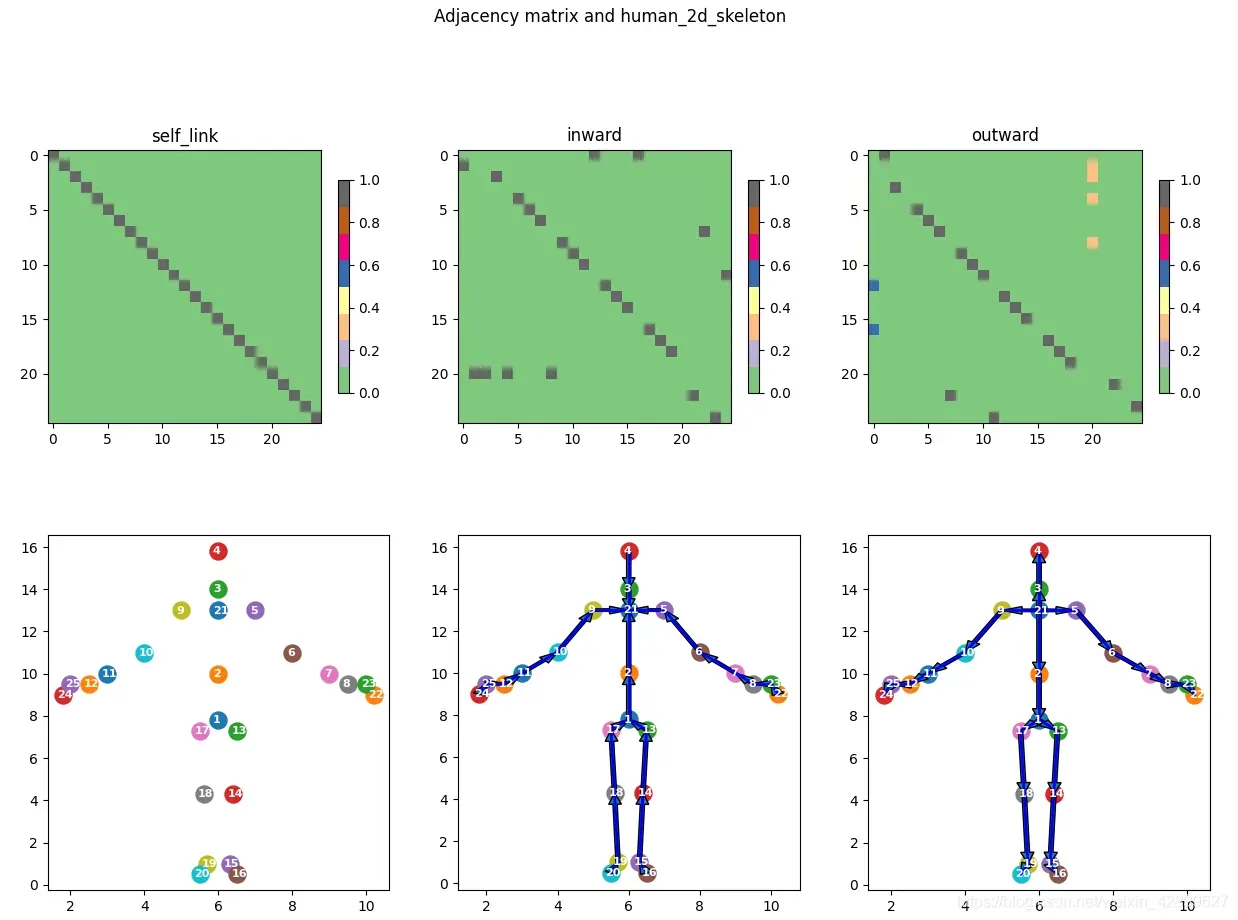
效果图
从左至右 依次为 sign_27_cvpr_0.png – I、 sign_27_cvpr_1.png – In、 sign_27_cvpr_2.png – Out、 sign_27_cvpr.png – All;其中 黄色像素表示 归一化过程中 该列 仅一个单元有值。
实现
基于 初始状态 可视化
tools.py
import numpy as np

def edge2mat(link, num_node):
    A = np.zeros((num_node, num_node))
    for i, j in link:
        A[j, i] = 1
    return A


def normalize_digraph(A):  # 除以每列的和
    Dl = np.sum(A, 0)
    h, w = A.shape
    Dn = np.zeros((w, w))
    for i in range(w):
        if Dl[i] > 0:
            Dn[i, i] = Dl[i] ** (-1)
    AD = np.dot(A, Dn)
    return AD


def get_spatial_graph(num_node, self_link, inward, outward):
    I = edge2mat(self_link, num_node)						# ex. (27, 27)
    In = normalize_digraph(edge2mat(inward, num_node))		# ex.(27, 27)
    Out = normalize_digraph(edge2mat(outward, num_node))	# ex.(27, 27)
    A = np.stack((I, In, Out))								# ex.(3, 27, 27)

    return A
sign_27_cvpr.py
from tools import get_spatial_graph


num_node = 27
self_link = [(i, i) for i in range(num_node)]  # 自旋图
inward_ori_index = [
                # (鼻子,眼睛)
                (5, 6), (5, 7),

                # (鼻子,肩膀)
                (5, 8), (5, 9),

                # 肩膀 - 手肘
                (8, 10), (9, 11),

                # 12-21 (-5) 7-16  左手
                (12,13),(12,14),(12,16),(12,18),(12,20),
                (14,15),(16,17),(18,19),(20,21),

                # 22-31 (-5) 17-26  右手
                (22,23),(22,24),(22,26),(22,28),(22,30),
                (24,25),(26,27),(28,29),(30,31),

                # (手肘, 手掌)
                (10,12),(11,22)]     # 5-31

inward = [(i - 5, j - 5) for (i, j) in inward_ori_index]   # (方向)向内   # 偏移5,可能是最小下标是5
outward = [(j, i) for (i, j) in inward]   # (方向)向外
neighbor = inward + outward  # 双向(邻近)


class Graph:
    def __init__(self, labeling_mode='spatial'):
        self.A = self.get_adjacency_matrix(labeling_mode)
        self.num_node = num_node
        self.self_link = self_link
        self.inward = inward
        self.outward = outward
        self.neighbor = neighbor

    def get_adjacency_matrix(self, labeling_mode=None):
        if labeling_mode is None:
            return self.A
        if labeling_mode == 'spatial':
            A = get_spatial_graph(num_node, self_link, inward, outward)
        else:
            raise ValueError()
        return A


if __name__ == '__main__':

    import matplotlib.pyplot as plt

    A = Graph('spatial').get_adjacency_matrix() # (3, 27, 27)

    # 逐层可视化
    for i in range(A.shape[0]):
        plt.imsave('sign_27_cvpr_{}.png'.format(i), A[i])  # (27, 27)

    # 整体可视化
    plt.imsave('sign_27_cvpr.png', A.transpose(1,2,0)) # (27, 27, 3)

	# 图像放大 -- 插值 (可选)
    import torch
    import torch.nn.functional as F
    x = F.interpolate(torch.from_numpy(A[None,...]), scale_factor=20, mode='nearest')   # torch.Size([1, 3, 540, 540])
    plt.imsave("scale.png", x.detach().numpy().squeeze().transpose(1,2,0)) # (540, 540, 3)
基于 预训练模型 获取 邻接矩阵
在 gcn-model.py中作如下修改:
 def forward(self, x):
        A = self.A.cuda(x.get_device())
        A_hands = self.A_hands.cuda(x.get_device())
        PA_hands = self.PA_hands.cuda(x.get_device())
        A = A + self.PA + A_hands * self.alpha + PA_hands * self.beta

        """"
        begin
        """
        # 保存 邻接矩阵A For 可视化
        tmpA = A.detach().cpu().numpy()
        n = 0
        while not os.path.exists("study/xxx_gcn_visual/9.npy"):  # 假设模型有10个block,输出前10次经过每个block的邻接矩阵
            if os.path.exists("study/xxx_gcn_visual/{}.npy".format(n)):
                n += 1
            else:
                break
        np.save("study/xxx_gcn_visual/{}.npy".format(n), tmpA)
        """
        end
        """

        y = None
        for i in range(self.num_subset):
            f = self.conv[i](x)
            N, C, T, V = f.size()
            z = torch.matmul(f.view(N, C * T, V), A[i]).view(N, C, T, V)
            y = z + y if y is not None else z

        y = self.bn(y)
        y += self.res(x)    # !!!
        return self.relu(y)
验证测试集指标 again 即可 ƪ(˘⌣˘)ʃ
batch_visual.py 批量可视化
import numpy as np
import os

root_dir = "xx_gcn_visual"

for root, dirs, files  in os.walk(root_dir):
    for A_file in files:
        if 'npy' in A_file:
            A_filepath = os.path.join(root, A_file)
            A_visual_filepath = os.path.splitext(A_filepath)[0] + ".png"
            A_visual_scale_filepath = os.path.splitext(A_filepath)[0] + "_scale.png"

            A_arr = np.load(A_filepath)  # (3, 27, 27)
            # print(A_arr.shape, A_arr.max(), A_arr.min())

            A_arr = (A_arr + abs(A_arr.min())) / (A_arr.max() - A_arr.min())
            print(A_arr.shape, A_arr.max(), A_arr.min())

            import matplotlib.pyplot as plt

            if len(A_arr.shape) == 3:	# ex. MS-AAGCN
                plt.imsave(A_visual_filepath, A_arr.transpose(1,2,0)) # (27, 27, 3)

                import torch
                import torch.nn.functional as F
                x = F.interpolate(torch.from_numpy(A_arr[None,...]), scale_factor=20, mode='nearest')   # torch.Size([1, 3, 540, 540])
                plt.imsave(A_visual_scale_filepath, x.detach().numpy().squeeze().transpose(1,2,0)) # (540, 540, 3)

            elif len(A_arr.shape) == 2:	# ex. ST-GCN

                plt.imsave(A_visual_filepath, A_arr) # (27, 27)

                import torch
                import torch.nn.functional as F
                x = F.interpolate(torch.from_numpy(A_arr[None,None,...]), scale_factor=20, mode='nearest')   # torch.Size([1, 1, 540, 540])
                plt.imsave(A_visual_scale_filepath, x.detach().numpy().squeeze()) # (540, 540)
相关链接

写在最后:若本文章对您有帮助,请点个赞啦 ٩(๑•̀ω•́๑)۶
文章出处登录后可见!
已经登录?立即刷新