全卷积网络FCN(Fully Convolutional Networks)是CV中语义分割任务的开山之作。FCN网络在PASCAL VOC(2012)数据集上获得了62.2%的mIoU。
论文全名《Fully Convolutional Networks for Semantic Segmentation》,发布于2015年CVPR。
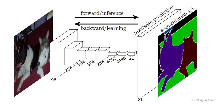
全卷积网络FCN
FCN亮点之一:全卷积
在以往的模型构建中,大部分研究者通常倾向于在卷积层后添加全连接层(FC,fully connected layer),以此来对特征进行映射和学习。而在FCN中,作者则摒弃了FC层,在整个模型架构中使用卷积层(Conv,Convolutional layer)来完成对图像特征的操作。
FCN亮点之二:反卷积deconvolution
反卷积可以理解为卷积的反向过程,通过不同步长的反卷积层实现不同的上采样操作。反卷积具体可以参考反卷积(Transposed Convolution)详细推导。
Note that the deconvolution fifilter in such a layer need not be fifixed (e.g., to bilinear upsampling), but can be learned. A stack of deconvolution layers and activation functions can even learn a nonlinear upsampling.文中提到:反卷积是可以学习的。可以使用双线性差值的核去初始化反卷积层,来加速学习。
FCN亮点之三:跳跃连接(skip connection)
在语义分割中不得不提的就是跳跃连接(skip connection)操作(见图2)。Skip connection允许模型在上采样过程中获得不同维度的特征,融合更多特征的同时也保留更多细节,帮助模型更精细的重建图像信息。
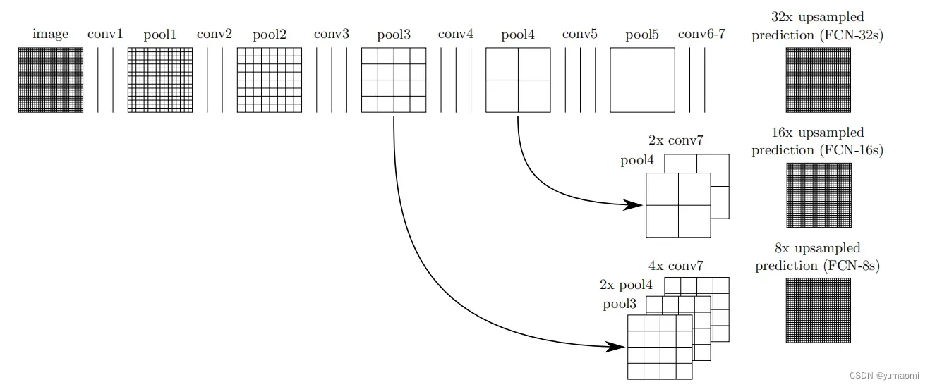
图2来自原论文,原作者分别构建了FCN-32、FCN-16和FCN-8三个模型,对于FCN-8,池化层pool3的输出分别于2倍上采样后的poo4的输出和4倍上采样后的conv7层的输出进行Concat操作(三个特征图在通道上进行相加),得到新的融合后的特征图(feature map)。再将这个特征图进行8倍上采样得到原图大小的特征图,至此,特征图即复原到原图大小,再经由后续操作即可完成语义分割任务。
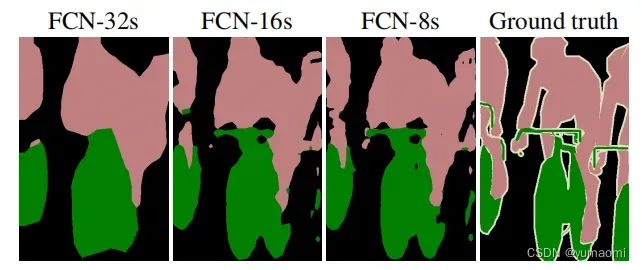
而FCN-16则只融合了pool4和con7两层特征,FCN-8则更加暴力,没有选择融合特征并直接将特征图上采样32倍到原图大小。这无疑损失了一定的精度,效果自然也显而易见地不如FCN-8来得精细(见图3)。
We address this by adding skips that combine the fifinal prediction layer with lower layers with fifiner strides. This turns a line topology into a DAG, with edges that skip ahead from lower layers to higher ones. As they see fewer pixels, the fifinerscalepredictions should need fewer layers, so it makes sense to make them from shallower net outputs. Combining fifine layers and coarse layers lets the model make local predictions that respect global structure. By analogy to the jet of Koenderick and van Doorn, we call our nonlinear feature hierarchy the deep jet.文中这段话说白了就是通过一个跳跃连接来精细化上采样,将最终的预测结果与较浅层的特征融合,让模型看到更多的像素,结合粗的特征和细的特征从而提升模型效果。
虽然FCN-8版本的分割效果并没有想象中的那么精细,但这在2015年已经是惊为天人的效果了。在语义分割的发展历史长河之中,FCN无疑是一个改变历史的网络,无论是全卷积的思想还是跳跃连接的思想,都在现在的各种语义分割模型中被广泛应用。
FCN的pytorch实现
因为原文基于Pascal VOC2012,所以这部分也以Pascal VOC2012为数据集,做一个复现工作。
首先导入一些基本模块
import cv2
import numpy as np
import matplotlib.pyplot as plt
from PIL import Image


import torch
import torch.nn as nn
import torch.optim as optim
import torch.nn.functional as F
from torch.utils.data import Dataset, DataLoader, random_split
from torchvision import transforms
from torchvision import models

from tqdm import tqdm
import warnings
读取VOC数据
VOC数据集中label的格式为P模式,需要通过VOC_COLORMAP映射到RGB格式。 这段内容改编自金渐层猫的博客内容。
import os
from PIL import Image
import numpy as np
import torch
from torch.utils.data import Dataset
from torchvision import transforms


VOC_COLORMAP = [[0, 0, 0], [128, 0, 0], [0, 128, 0], [128, 128, 0],
                [0, 0, 128], [128, 0, 128], [0, 128, 128], [128, 128, 128],
                [64, 0, 0], [192, 0, 0], [64, 128, 0], [192, 128, 0],
                [64, 0, 128], [192, 0, 128], [64, 128, 128], [192, 128, 128],
                [0, 64, 0], [128, 64, 0], [0, 192, 0], [128, 192, 0],
                [0, 64, 128]]

VOC_CLASSES = ['background', 'aeroplane', 'bicycle', 'bird', 'boat',
               'bottle', 'bus', 'car', 'cat', 'chair', 'cow',
               'diningtable', 'dog', 'horse', 'motorbike', 'person',
               'potted plant', 'sheep', 'sofa', 'train', 'tv/monitor']

colormap2label = torch.zeros(256 ** 3, dtype=torch.uint8)
for i, colormap in enumerate(VOC_COLORMAP):
    colormap2label[(colormap[0] * 256 + colormap[1]) * 256 + colormap[2]] = i


def voc_label_indices(colormap):
    """
    convert colormap (PIL image) to colormap2label (uint8 tensor).
    """
    colormap = np.array(colormap).astype('int32')
    idx = ((colormap[:, :, 0] * 256 + colormap[:, :, 1]) * 256
           + colormap[:, :, 2])
    return colormap2label[idx]


def read_file_list(root, is_train=True):
    txt_fname = root + '/ImageSets/Segmentation/' + ('train.txt' if is_train else 'val.txt')
    with open(txt_fname, 'r') as f:
        filenames = f.read().split()
    images = [os.path.join(root, 'JPEGImages', i + '.jpg') for i in filenames]
    labels = [os.path.join(root, 'SegmentationClass', i + '.png') for i in filenames]
    return images, labels  # file list


def voc_rand_crop(image, label, height, width):
    """
    Random crop image (PIL image) and label (PIL image).
    """
    i, j, h, w = transforms.RandomCrop.get_params(
        image, output_size=(height, width))

    image = transforms.functional.crop(image, i, j, h, w)
    label = transforms.functional.crop(label, i, j, h, w)

    return image, label


class VOCSegDataset(torch.utils.data.Dataset):
    def __init__(self, is_train, crop_size, voc_root):
        """
        crop_size: (h, w)
        """
        self.transform = transforms.Compose([
            transforms.ToTensor(),
            #transforms.Normalize(mean=self.rgb_mean, std=self.rgb_std)
        ])

        self.crop_size = crop_size  # (h, w)
        images, labels = read_file_list(root=voc_root, is_train=is_train)
        self.images = self.filter(images)  # images list
        self.labels = self.filter(labels)  # labels list
        print('Read ' + str(len(self.images)) + ' valid examples')

    def filter(self, imgs):  # 过滤掉尺寸小于crop_size的图片
        return [img for img in imgs if (
                Image.open(img).size[1] >= self.crop_size[0] and
                Image.open(img).size[0] >= self.crop_size[1])]

    def __getitem__(self, idx):
        image = self.images[idx]
        label = self.labels[idx]
        image = Image.open(image).convert('RGB')
        label = Image.open(label).convert('RGB')
        image, label = voc_rand_crop(image, label,
                                     *self.crop_size)
        image = self.transform(image)
        label = voc_label_indices(label)
        return image, label  # float32 tensor, uint8 tensor

    def __len__(self):
        return len(self.images)
构建数据集
voc_train = VOCSegDataset(is_train = True, crop_size=(224,224), voc_root = 'dataset/VOCdevkit/VOC2012/')
voc_val = VOCSegDataset(is_train = False, crop_size=(224,224), voc_root = 'dataset/VOCdevkit/VOC2012/')
也可以打印一下数据集img和label,其中img是图像数据,label是label标签
for i, (img, label) in enumerate(voc_train):
    plt.figure(figsize=(10,10))
    plt.subplot(221)
    plt.imshow(img.moveaxis(0,2))
    plt.subplot(222)
    plt.imshow(label)
    plt.show()
    plt.close()
    if i ==1:
        break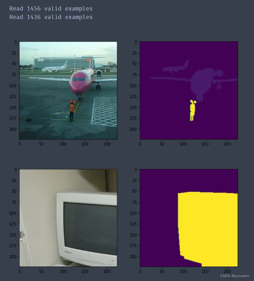
构建FCN-8模型
class FCN8(nn.Module):
    def __init__(self, num_classes):
        super(FCN8, self).__init__()
        self.stage1 = nn.Sequential(
            nn.Conv2d(in_channels=3,out_channels=96,kernel_size=3,padding=1),
            nn.ReLU(),
            nn.BatchNorm2d(num_features=96),
            nn.MaxPool2d(kernel_size=2,padding=0)
        )
        self.stage2 = nn.Sequential(
            nn.Conv2d(in_channels=96,out_channels=256,kernel_size=3,padding=1),
            nn.ReLU(),
            nn.BatchNorm2d(num_features=256),
            nn.MaxPool2d(kernel_size=2,padding=0)
        )

        self.stage3 = nn.Sequential(
            nn.Conv2d(in_channels=256,out_channels=384,kernel_size=3,padding=1),
            nn.ReLU(),
            nn.BatchNorm2d(num_features=384),

            nn.Conv2d(in_channels=384,out_channels=384,kernel_size=3,padding=1),
            nn.ReLU(),
            nn.BatchNorm2d(num_features=384),

            nn.Conv2d(in_channels=384,out_channels=256,kernel_size=3,padding=1),
            nn.ReLU(),
            nn.BatchNorm2d(num_features=256),

            nn.MaxPool2d(kernel_size=2,padding=0)
        )

        self.stage4 = nn.Sequential(
            nn.Conv2d(in_channels=256,out_channels=512,kernel_size=3,padding=1),
            nn.ReLU(),
            nn.BatchNorm2d(num_features=512),

            nn.Conv2d(in_channels=512,out_channels=512,kernel_size=3,padding=1),
            nn.ReLU(),
            nn.BatchNorm2d(num_features=512),

            nn.MaxPool2d(kernel_size=2,padding=0)
        )

        self.stage5 = nn.Sequential(
            nn.Conv2d(in_channels=512,out_channels=num_classes,kernel_size=3,padding=1),
            nn.ReLU(),
            nn.BatchNorm2d(num_features=num_classes),

            nn.MaxPool2d(kernel_size=2,padding=0)
        )

        #k倍上采样
        self.upsample_2 = nn.ConvTranspose2d(in_channels=512, out_channels=512, kernel_size=4, padding= 1,stride=2)
        self.upsample_4 = nn.ConvTranspose2d(in_channels=num_classes, out_channels=num_classes, kernel_size=4, padding= 0,stride=4)
        self.upsample_81 = nn.ConvTranspose2d(in_channels=512+num_classes+256, out_channels=512+num_classes+256, kernel_size=4, padding= 0,stride=4)
        self.upsample_82 = nn.ConvTranspose2d(in_channels=512+num_classes+256, out_channels=512+num_classes+256, kernel_size=4, padding= 1,stride=2)
        #最后的预测模块
        self.final = nn.Sequential(
            nn.Conv2d(512+num_classes+256, num_classes, kernel_size=7, padding=3),
        )

    def forward(self, x):
        x = x.float()
        #conv1->pool1->输出
        x = self.stage1(x)
        #conv2->pool2->输出
        x = self.stage2(x)
        #conv3->pool3->输出输出, 经过上采样后, 需要用pool3暂存
        x = self.stage3(x)
        pool3 = x
        #conv4->pool4->输出输出, 经过上采样后, 需要用pool4暂存
        x = self.stage4(x)
        pool4 = self.upsample_2(x)

        x = self.stage5(x)
        conv7 = self.upsample_4(x)

        #对所有上采样过的特征图进行concat, 在channel维度上进行叠加
        x = torch.cat([pool3, pool4, conv7], dim = 1)
        #经过一个分类网络,输出结果(这里采样到原图大小,分别一次2倍一次4倍上采样来实现8倍上采样)
        output = self.upsample_81(x)
        output = self.upsample_82(output)
        output = self.final(output)

        return output
训练模型
#创建dataloader
dataloader_train = DataLoader(voc_train, batch_size = 16, shuffle=True,)
dataloader_val = DataLoader(voc_val, batch_size = 16)
#损失函数选用多分类交叉熵损失函数
lossf = nn.CrossEntropyLoss()
#PascalVOC2012  一共20类+1类背景
model = FCN8(num_classes=21)
#选用adam优化器来训练
optimizer = optim.SGD(model.parameters(),lr=0.1)
#训练50轮
epochs_num = 50
这里借用了d2l库中的train函数
可以通过pip install d2l安装
from d2l import torch as d2l
def train_ch13(net, train_iter, test_iter, loss, trainer, num_epochs,
               devices=d2l.try_all_gpus()):
    """Train a model with mutiple GPUs (defined in Chapter 13).
    Defined in :numref:`sec_image_augmentation`"""
    timer, num_batches = d2l.Timer(), len(train_iter)
    animator = d2l.Animator(xlabel='epoch', xlim=[1, num_epochs], ylim=[0, 1],
                            legend=['train loss', 'train acc', 'test acc'])
    net = nn.DataParallel(net, device_ids=devices).to(devices[0])
    for epoch in range(num_epochs):
        # Sum of training loss, sum of training accuracy, no. of examples,
        # no. of predictions
        metric = d2l.Accumulator(4)
        for i, (features, labels) in enumerate(dataloader_train):
            timer.start()
            l, acc = d2l.train_batch_ch13(
                net, features, labels.long(), loss, trainer, devices)
            metric.add(l, acc, labels.shape[0], labels.numel())
            timer.stop()
            if (i + 1) % (num_batches // 5) == 0 or i == num_batches - 1:
                animator.add(epoch + (i + 1) / num_batches,
                             (metric[0] / metric[2], metric[1] / metric[3],
                              None))
        test_acc = d2l.evaluate_accuracy_gpu(net, test_iter)
        animator.add(epoch + 1, (None, None, test_acc))
        print(f'loss {metric[0] / metric[2]:.3f}, train acc '
              f'{metric[1] / metric[3]:.3f}, test acc {test_acc:.3f}')
        print(f'{metric[2] * num_epochs / timer.sum():.1f} examples/sec on '
              f'{str(devices)}')

train_ch13(model, dataloader_train, dataloader_val, lossf, optimizer,epochs_num)
最终acc约为63.3%。
总结
本文构建了最为简单的FCN网络模型,简单复现了FCN论文中的部分结果。如果使用resnet替换为FCN的backbone,模型的效果还会更好。
文章出处登录后可见!