1. Unit 1: Review of probability

1.1 stochastic and state space

状态空间就是所有可能取值

1.2 Bayesian vs Frequentist （goodnotes）

1.3 离散分布

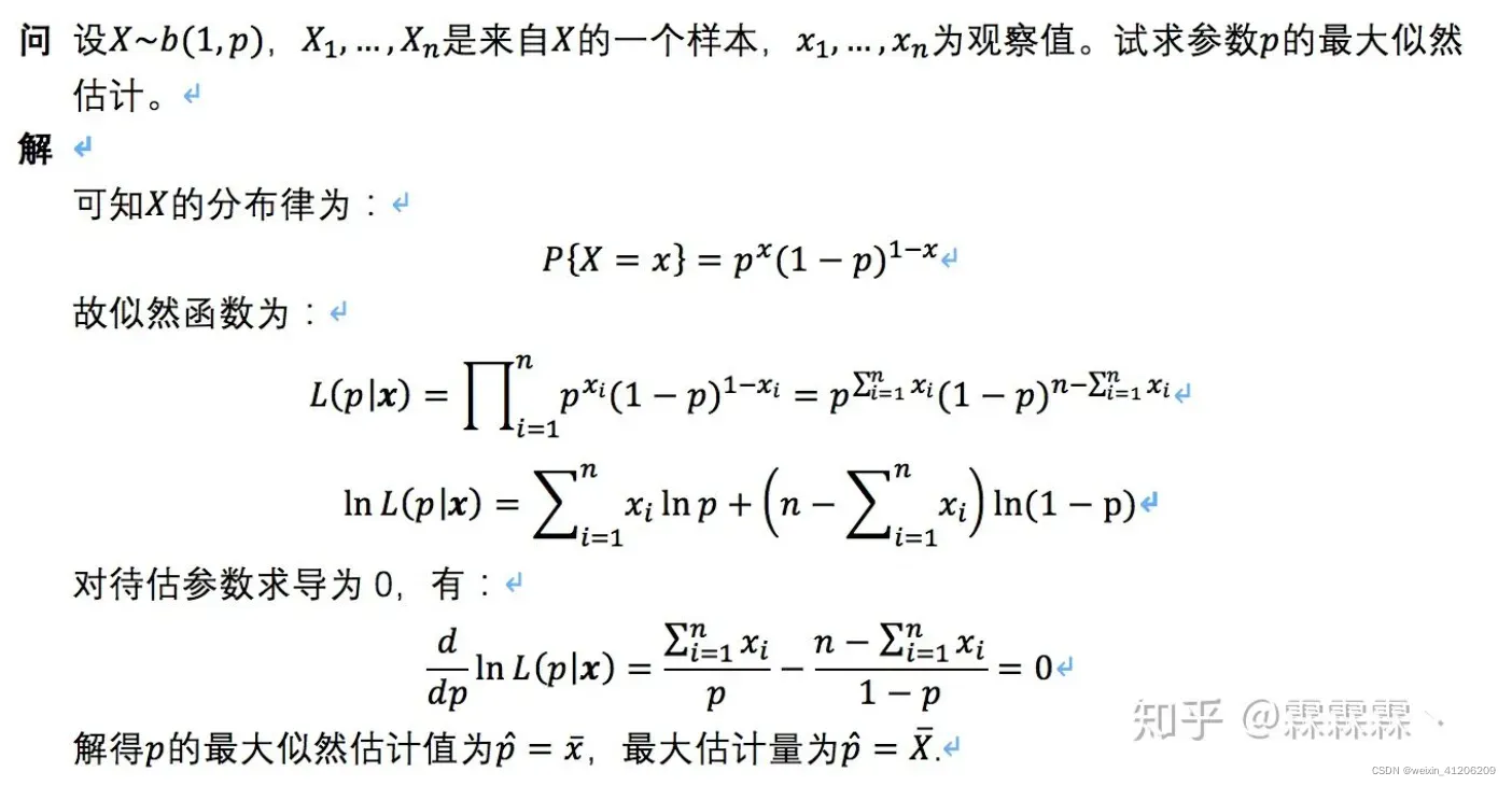
• 伯努利分布（Bernoulli）：即0-1分布
• 二项分布（Binomial）：即n重伯努利实验
• 中心极限定理（Central Limited Theorem）（goodnotes）

1.4 连续分布

• 概率密度函数
• 均匀分布（Uniform）
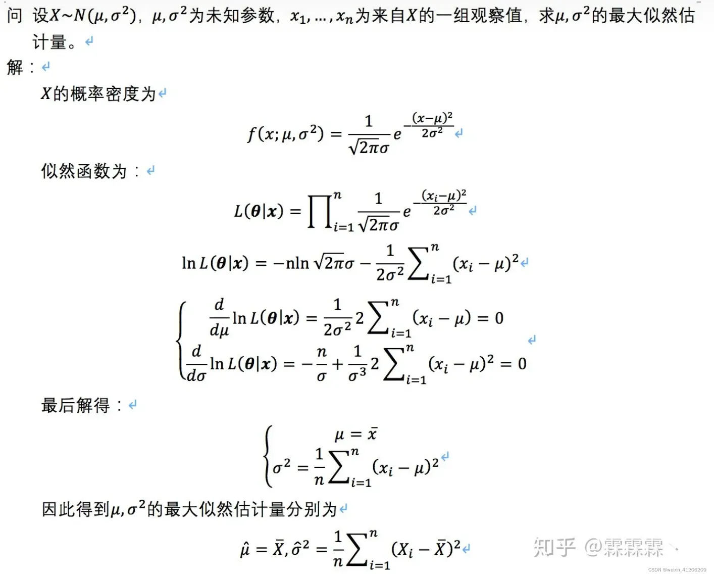
• 高斯/正态分布（Gaussian）

1.5 最大似然估计（MLE）

• 独立同分布（idd）

• 离散型随机变量MLE
  

• 连续型随机变量MLE
  

• 联合概率，边缘概率，条件概率

1.6 贝叶斯定理（Baye’s Rule）

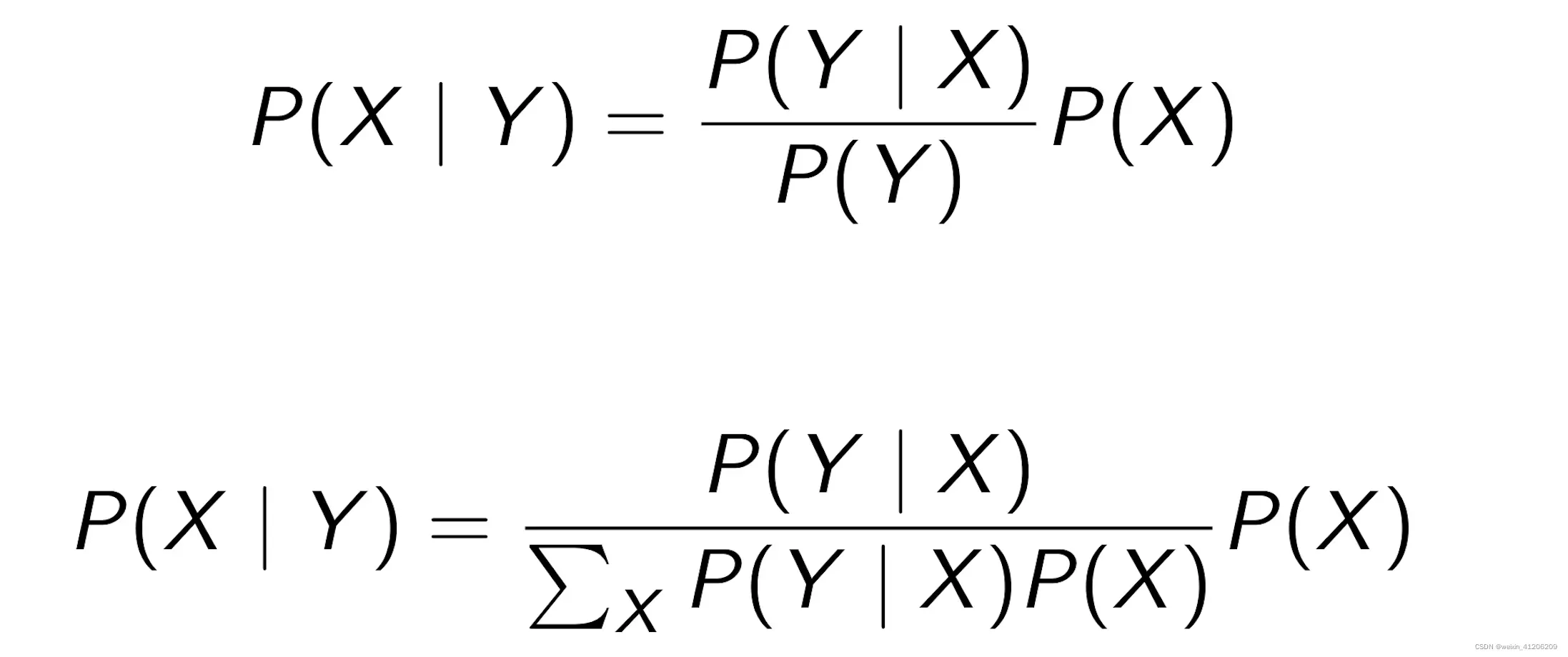
P(H) 是先验概率
P(D|H)是似然函数
P(H|D)是后验概率

1.8 信息论

• 信息熵

信息熵越大，说明不确定信息越多。所以，越随机，信息熵越大。
事件发生的概率越高，所携带的信息熵越低，即该事件并没有消除任何的不确定性。

• 微分熵（对于连续变量）
  

• 交叉熵
  
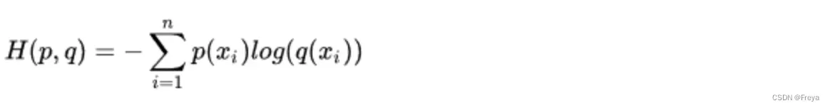
  用错误分布q来表示真实分布p的平均编码长度（对比信息熵），

• KL散度

  当p不固定时（即不知p(x)），使用另一种度量方式来度量两个分布之间的差异，相对熵，将由q得到的平均编码长度比由p得到的平均编码长度多出的bit数成为KL散度。
  
  注意：KL散度的不对称性，它不是不同分布间距离的度量，即用p近似q和用q近似p，二者所得的损失信息并不是一样的。

• 交叉熵与KL散度的关系
  
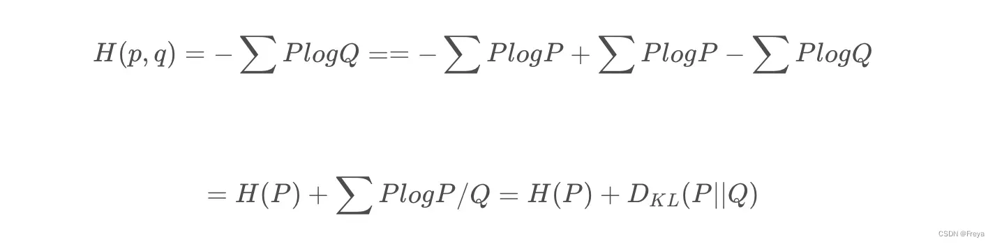
  交叉熵就是真实分布的熵H( P)与KL散度的和，最小化交叉熵与最小化KL散度是一样的。
  由杰森不等式可得，只有当p=q时，KL散度才=0.

2. Unit 2: Linear Regression, Bayesian and Frequentists version

2.1 Multivariate Gaussian distribution

• PDF（概率密度函数）和CDF（累积分布函数）的区别 readerP5
  CDF即PDF的积分
• 马氏距离和欧式距离的区别 readerP9
• covariance matrix 的三种形式 unit2 slide1 P7
• 谱分解(spectral decomposition) readerP10
  谱分解就是特征分解，将矩阵分解为由其特征值和特征向量表示的矩阵之积的方法。需要注意只有对可对角化矩阵才可以施以特征分解。
  应用 unit2 slide1 P23
• MLE for MV Gaussian distribution unit2 slide1 P20

2.2 Linear Regression

• 线性回归的定义 goodnotes ML P4

  线性回归和非线性回归的区别：It is important to realise that all examples of this section are lin- ear regression, even if we fit a non linear function to the data. The distinction between linear and non linear regression is not whether or not to use of linear functions to model the data, but whether the fit function is a linear function its weights.

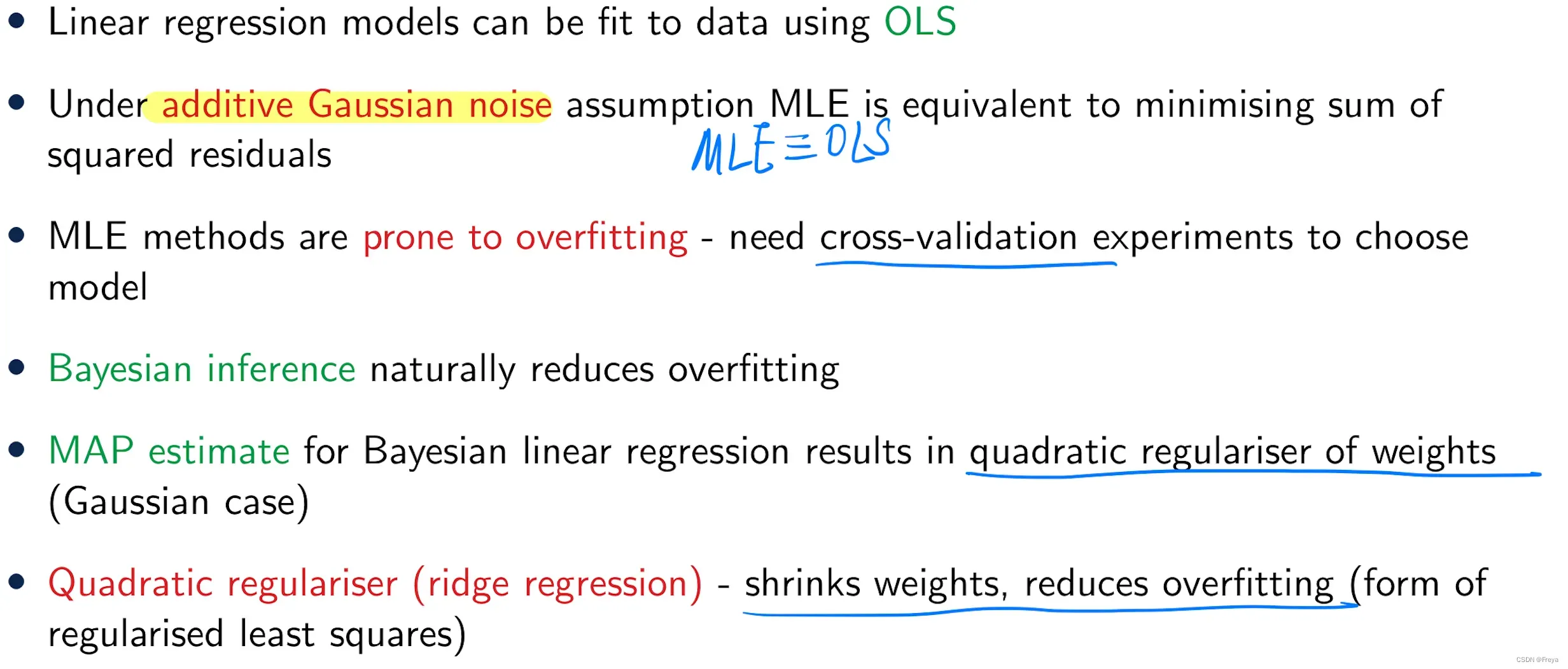
• OLS（普通最小二乘法）和MLE（最大似然估计法）的区别

  目的都是根据一些给定的样本（x, y）对参数（w, θ）进行估计。该参数带入回归方程中可以很好地拟合训练样本，也可以输入新样本，得到预测值。

  OLS的思想是要使得target和pred的残差平方和最小，而MLE的思想是通过求得出target最大概率的参数值。

  likelihood似然函数就是概率分布函数，所以，最大似然法需要已知这个dataset的概率分布函数。在distribution为高斯分布时，OLS和MLE等价（即OLS不考虑任何noise，MLE考虑Gaussian noise）。

  公式见 unit2 slide2 P25

• OLS推导过程 unit2 slide2 P7

• over-fitting / under-fitting——cross-validation

2.3 Bayesian Linear Regression

• 贝叶斯线性回归与线性回归的区别 goodnotes ML P4
  贝叶斯线性回归不再只是求模型参数的最佳值，而是求模型参数的后验分布，且引入了先验分布

• Bayesian methods are less prone to overfitting than MLE estimates

• Competing the square unit2 slide3 P12

• Bayesian vs MLE vs MAP readerP25
  MAP公式 unit2 slide5 P5

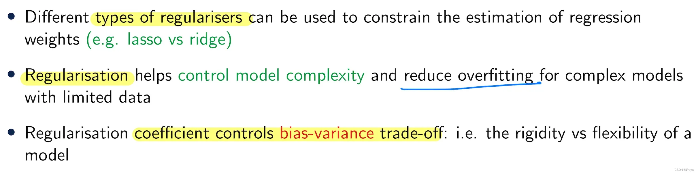
• Regularisation unit2 slide5 P6
  second term——penalty term for large weights

• Lasso vs Ridge unit2 slide5 P11

  通过限制（constraining）或缩减(shrinking)方法牺牲偏差（bias）显著减小方差（variance），可以提高模型在测试样本集上的准确率。

  Ridge回归（二次项时是Ridge回归，q = 2） unit2 slide5 P9
  q = 1时是Lasso回归。

  Ridge回归的一个显著劣势在于：最终模型始终包括全部p个变量。惩罚项可以将系数往0方向缩减，但是不会确切地压缩到0。这种设定不影响预测精度，但是当变量p非常大时，不便于模型解释。

  Ridge 和 Lasso最大的区别在于，当 lamda变得很大时，Lasso 回归中某些参数（也就是w ）会变为0.

• Summarisation
  

• OLS和Bayesian linear regression的区别

  OLS, which is a MLE of model parameters in linear regression under the assumption of a Gaussian noise model. We have seen that OLE corresponds to the minimisation of a loss function.

  In Bayesian linear regression, we minimise the same loss function but a penalty term is introduced that discourages the model parameters from being large, which is called a regularisation term.

3. Unit 3: Logistic Regression and Introduction to Neural Networks

3.1 Introduction of NN

• Logistic Regression

  逻辑回归的模型是一个非线性模型，sigmoid函数，又称逻辑回归函数。但是它本质上又是一个线性回归模型，因为除去sigmoid映射函数关系，其他的步骤，算法都是线性回归的。可以说，逻辑回归，都是以线性回归为理论支持的。

  逻辑回归不像线性回归可以通过具体结果来找参，只能解出近似解（非线性）。

• perceptron

  感知机模型和逻辑回归的区别：感知机是用阶跃函数（sign()）来控制输出二级信号，逻辑回归是用sigmoid函数。

  感知机
  
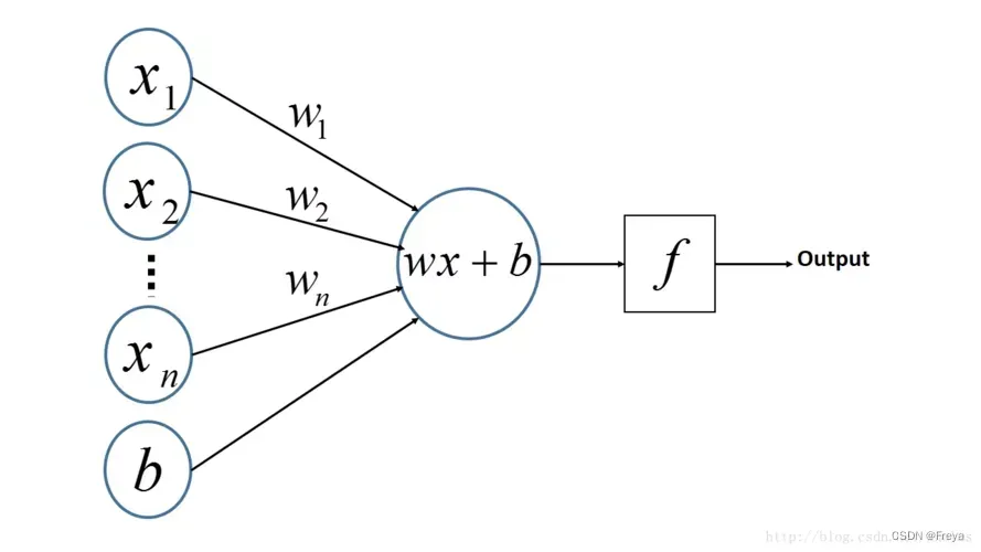
  PLA（感知机算法）：
  
  Add & Subtract unit3 slide51P15
  思想：If the classification is correct, leave the weights alone, otherwise add or subtract the input pattern so that the weights may do better on the same pattern next time around. If data is linearly separable, the perceptron algorithm will find a set of weights that separates the two classes.

  proof of perceptron theorem unit3 slide1 P19

  limitation of perception unit3 slide1 P23

  loss function of perception reader3-1 P26

3.2 Logistic Regression

• minimise the loss function unit3 slide2 P8

• SGD(最速梯度下降) unit3 slide2 P9
  SGD的好处 reader3-1 P31
  但SGD可能会lead a very slow convergence, 解决办法 reader3-1 P33

• 为什么逻辑回归中用KL（或者交叉熵）不用MSE？ unit3 slide3 P14
  原因一，使用交叉熵loss下降的更快；
  原因二，使用交叉熵是凸优化，MSE是非凸优化。

  线性回归（回归问题）使用的是平方损失（MSE）：

  因为这个函数 是凸函数，直接求导等于零，即可求出解析解，很简单。但是对于逻辑回归则不行（分类问题）【注意：逻辑回归不是回归！是分类！！】。因为如果逻辑回归也用平方损失作为损失函数，则：

  其中 表示样本数量。
  上式是非凸的，不能直接求解析解，而且不宜优化，易陷入局部最优解，即使使用梯度下降也很难得到全局最优解。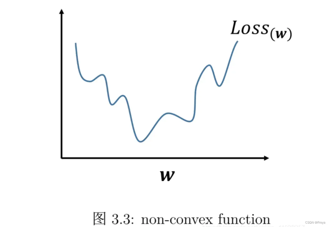

  

• Bayesian Logistic Regression的困境

  But it does mean that the posterior cannot be expressed as a Gaussian. This means that the posterior cannot neatly be presented as a parameterised distribution whose parameters can be calculated in a neat formula. Even if you were able to find a closed analytical expression for the posterior, in prediction you would have to marginalise the weights, which would lead to nasty multi-dimensional integrals.

4. Unit 4: Decision Trees, Random Forest, Boosting

4.1 DTs

• DTs的优劣 unit4 slide1 P11
  DTs are built by greedy, top-down, recursive partitioning of the feature space
  选信息增益大的作为判断标准。

• ID3划分的例子 unit4 slide1 P22

• CART划分的例子 unit4 slide2 P12
  CART算连续的 unit4 slide2 P14

• Confusion matrix ai goodnotes
  ROC-AUC unit4 slide2 P23

4.2 Regression Trees Ensembles

• regularisation for DTs unit4 slide3 P8

• Bagging即套袋法
  Bootstraping，即自助法：它是一种有放回的抽样方法（可能抽到重复的样本）。

• Boosting
  其主要思想是将弱分类器组装成一个强分类器。在PAC（概率近似正确）学习框架下，则一定可以将弱分类器组装成一个强分类器。

  关于Boosting的两个核心问题：

  1）在每一轮如何改变训练数据的权值或概率分布？

  通过提高那些在前一轮被弱分类器分错样例的权值，减小前一轮分对样例的权值，来使得分类器对误分的数据有较好的效果。

  2）通过什么方式来组合弱分类器？

  通过加法模型将弱分类器进行线性组合，比如AdaBoost通过加权多数表决的方式，即增大错误率小的分类器的权值，同时减小错误率较大的分类器的权值。

  而提升树通过拟合残差的方式逐步减小残差，将每一步生成的模型叠加得到最终模型。

  其算法过程如下：

  A）从原始样本集中抽取训练集。每轮从原始样本集中使用Bootstraping的方法抽取n个训练样本（在训练集中，有些样本可能被多次抽取到，而有些样本可能一次都没有被抽中）。共进行k轮抽取，得到k个训练集。（k个训练集之间是相互独立的）

  B）每次使用一个训练集得到一个模型，k个训练集共得到k个模型。（注：这里并没有具体的分类算法或回归方法，我们可以根据具体问题采用不同的分类或回归方法，如决策树、感知器等）

  C）对分类问题：将上步得到的k个模型采用投票的方式得到分类结果；对回归问题，计算上述模型的均值作为最后的结果。（所有模型的重要性相同）

• 两种ensemble methods: boosting & bagging unit4 slide4 P5
  Bagging和Boosting的区别：

  1）样本选择上：

  Bagging：训练集是在原始集中有放回选取的，从原始集中选出的各轮训练集之间是独立的。
  Boosting：每一轮的训练集不变，只是训练集中每个样例在分类器中的权重发生变化。而权值是根据上一轮的分类结果进行调整。

  2）样例权重：

  Bagging：使用均匀取样，每个样例的权重相等
  Boosting：根据错误率不断调整样例的权值，错误率越大则权重越大。
  3）预测函数：
  Bagging：所有预测函数的权重相等。
  Boosting：每个弱分类器都有相应的权重，对于分类误差小的分类器会有更大的权重。

  4）并行计算：
  Bagging：各个预测函数可以并行生成
  Boosting：各个预测函数只能顺序生成，因为后一个模型参数需要前一轮模型的结果。

• RF是怎么降低variance的 unit4 slide4 P9

• AdaBoost unit4 slide4 P12

• Gradient Boosted Trees unit4 slide4 P16

• XGBoost unit4 slide4 P17

5. Unit 5: Mixture Models, E/M Algorithm

5.1 GMM

• latent variable

• k-means的缺点 reader5 P14 、unit5 slide1 P10
  K-means is an example of E/M optimisation

• GMM即两步 unit5 slide1 P12

• EM for GMM unit5 slide1 P22

• ELBO