【人工智能作业】3-例题程序复现 PyTorch版

1.使用pytorch复现课上例题

代码如下

import torch

x1, x2 = torch.Tensor([0.5]), torch.Tensor([0.3])
y1, y2 = torch.Tensor([0.23]), torch.Tensor([-0.07])
print("=====输入值：x1, x2；真实输出值：y1, y2=====")
print(x1, x2, y1, y2)
w1, w2, w3, w4, w5, w6, w7, w8 = torch.Tensor([0.2]), torch.Tensor([-0.4]), torch.Tensor([0.5]), torch.Tensor(
    [0.6]), torch.Tensor([0.1]), torch.Tensor([-0.5]), torch.Tensor([-0.3]), torch.Tensor([0.8])  # 权重初始值
w1.requires_grad = True
w2.requires_grad = True
w3.requires_grad = True
w4.requires_grad = True
w5.requires_grad = True
w6.requires_grad = True
w7.requires_grad = True
w8.requires_grad = True


def sigmoid(z):
    a = 1 / (1 + torch.exp(-z))
    return a


def forward_propagate(x1, x2):
    in_h1 = w1 * x1 + w3 * x2
    out_h1 = sigmoid(in_h1)  # out_h1 = torch.sigmoid(in_h1)
    in_h2 = w2 * x1 + w4 * x2
    out_h2 = sigmoid(in_h2)  # out_h2 = torch.sigmoid(in_h2)

    in_o1 = w5 * out_h1 + w7 * out_h2
    out_o1 = sigmoid(in_o1)  # out_o1 = torch.sigmoid(in_o1)
    in_o2 = w6 * out_h1 + w8 * out_h2
    out_o2 = sigmoid(in_o2)  # out_o2 = torch.sigmoid(in_o2)

    print("正向计算：o1 ,o2")
    print(out_o1.data, out_o2.data)

    return out_o1, out_o2


def loss_fuction(x1, x2, y1, y2):  # 损失函数
    y1_pred, y2_pred = forward_propagate(x1, x2)  # 前向传播
    loss = (1 / 2) * (y1_pred - y1) ** 2 + (1 / 2) * (y2_pred - y2) ** 2  # 考虑 ： t.nn.MSELoss()
    print("损失函数（均方误差）：", loss.item())
    return loss


def update_w(w1, w2, w3, w4, w5, w6, w7, w8):
    # 步长
    step = 1
    w1.data = w1.data - step * w1.grad.data
    w2.data = w2.data - step * w2.grad.data
    w3.data = w3.data - step * w3.grad.data
    w4.data = w4.data - step * w4.grad.data
    w5.data = w5.data - step * w5.grad.data
    w6.data = w6.data - step * w6.grad.data
    w7.data = w7.data - step * w7.grad.data
    w8.data = w8.data - step * w8.grad.data
    w1.grad.data.zero_()  # 注意：将w中所有梯度清零
    w2.grad.data.zero_()
    w3.grad.data.zero_()
    w4.grad.data.zero_()
    w5.grad.data.zero_()
    w6.grad.data.zero_()
    w7.grad.data.zero_()
    w8.grad.data.zero_()
    return w1, w2, w3, w4, w5, w6, w7, w8


if __name__ == "__main__":

    print("=====更新前的权值=====")
    print(w1.data, w2.data, w3.data, w4.data, w5.data, w6.data, w7.data, w8.data)

    for i in range(1000):
        print("=====第" + str(i) + "轮=====")
        L = loss_fuction(x1, x2, y1, y2)  # 前向传播，求 Loss，构建计算图
        L.backward()  # 自动求梯度，不需要人工编程实现。反向传播，求出计算图中所有梯度存入w中
        print("\tgrad W: ", round(w1.grad.item(), 2), round(w2.grad.item(), 2), round(w3.grad.item(), 2),
              round(w4.grad.item(), 2), round(w5.grad.item(), 2), round(w6.grad.item(), 2), round(w7.grad.item(), 2),
              round(w8.grad.item(), 2))
        w1, w2, w3, w4, w5, w6, w7, w8 = update_w(w1, w2, w3, w4, w5, w6, w7, w8)

    print("更新后的权值")
    print(w1.data, w2.data, w3.data, w4.data, w5.data, w6.data, w7.data, w8.data)

训练前参数为（图片文字过小，使用文本）

 =====输入值：x1, x2；真实输出值：y1, y2=====
tensor([0.5000]) tensor([0.3000]) tensor([0.2300]) tensor([-0.0700])
=====更新前的权值=====
tensor([0.2000]) tensor([-0.4000]) tensor([0.5000]) tensor([0.6000]) tensor([0.1000]) tensor([-0.5000]) tensor([-0.3000]) tensor([0.8000])

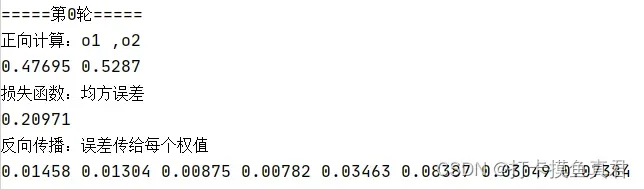
 第一轮运行结果如下

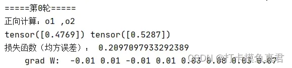
作业二中的第一轮运行结果

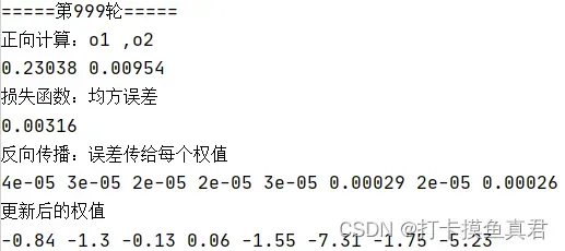
第一千轮运行结果如下（图片文字过小，使用文本） 

 =====第999轮=====
正向计算：o1 ,o2
tensor([0.2296]) tensor([0.0098])
损失函数（均方误差）： 0.0031851977109909058
    grad W:  -0.0 -0.0 -0.0 -0.0 -0.0 0.0 -0.0 0.0
更新后的权值
tensor([1.6515]) tensor([0.1770]) tensor([1.3709]) tensor([0.9462]) tensor([-0.7798]) tensor([-4.2741]) tensor([-1.0236]) tensor([-2.1999])

 作业二中第一千轮运行结果

2.对比【作业3】和【作业2】的程序，观察两种方法结果是否相同？如果不同，哪个正确？

结果不相同，作业三正确。 

3.【作业2】程序更新（保留【作业2中】的错误答案，留作对比。新程序到作业3）

 更新后的反向传播函数代码

def back_propagate(out_o1, out_o2, out_h1, out_h2):
    # 反向传播
    d_o1 = out_o1 - y1
    d_o2 = out_o2 - y2

    d_w5 = d_o1 * out_o1 * (1 - out_o1) * out_h1
    d_w7 = d_o1 * out_o1 * (1 - out_o1) * out_h2
    d_w6 = d_o2 * out_o2 * (1 - out_o2) * out_h1
    d_w8 = d_o2 * out_o2 * (1 - out_o2) * out_h2

    d_w1 = (d_o1 * out_h1 * (1 - out_h1) * w5 + d_o2 * out_o2 * (1 - out_o2) * w6) * out_h1 * (1 - out_h1) * x1
    d_w3 = (d_o1 * out_h1 * (1 - out_h1) * w5 + d_o2 * out_o2 * (1 - out_o2) * w6) * out_h1 * (1 - out_h1) * x2
    d_w2 = (d_o1 * out_h1 * (1 - out_h1) * w7 + d_o2 * out_o2 * (1 - out_o2) * w8) * out_h2 * (1 - out_h2) * x1
    d_w4 = (d_o1 * out_h1 * (1 - out_h1) * w7 + d_o2 * out_o2 * (1 - out_o2) * w8) * out_h2 * (1 - out_h2) * x2

    print("w的梯度:", round(d_w1, 2), round(d_w2, 2), round(d_w3, 2), round(d_w4, 2), round(d_w5, 2), round(d_w6, 2),
          round(d_w7, 2), round(d_w8, 2))

    return d_w1, d_w2, d_w3, d_w4, d_w5, d_w6, d_w7, d_w8

4. 对比【作业2】与【作业3】的反向传播的实现方法。总结并陈述

作业2中的方法通过手动计算，得到反向传播过程中各参数梯度。作业3通过张量Tensor求Loss，构建计算图，在最后通过backword()自动求梯度。由于使用了Pytorch当中的Tensor张量，使用前向传播建立计算图，即可根据传播结果利用back_propagate自动计算梯度。激活函数使用Pytorch自带的torch.sigmoid()。

5.激活函数Sigmoid用PyTorch自带函数torch.sigmoid()，观察、总结并陈述

二者使用同一个公式

但PyTorch自带函数时间效率更高 。

6.激活函数Sigmoid改变为Relu，观察、总结并陈述  

线性整流函数（Linear rectification function）,又称修正线性单元，是一种人工神经网络中常用的激活函数（activation function），通常指代以斜坡函数及其变种为代表的非线性函数。 

 Relu函数公式为

 使用Relu函数时间效率并无较大变化，但结果出现改变。

 7.损失函数MSE用PyTorch自带函数 t.nn.MSELoss()替代，观察、总结并陈述

 MSE是mean squared error的缩写，即平均平方误差，简称均方误差。

MSE是逐元素计算的，公式为

使用 t.nn.MSELoss()函数替代结果发生改变，但变化幅度小于使用Relu函数。

8.损失函数MSE改变为交叉熵，观察、总结并陈述 

交叉熵（Cross Entropy）是香农信息论中一个重要概念，主要用于度量两个概率分布间的差异性信息。语言模型的性能通常用交叉熵和复杂度来衡量。

 交叉熵公式为

 其中y代表真实值分类（0或1），a代表预测值，交叉熵值越小，预测结果越准。

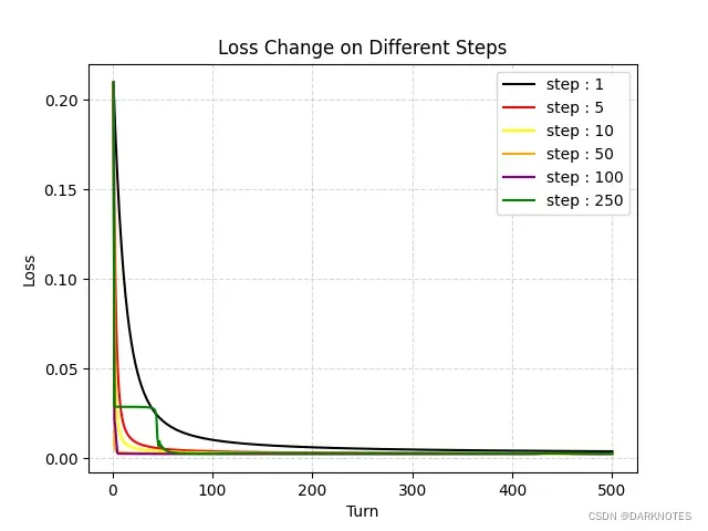
9.改变步长，训练次数，观察、总结并陈述。

每次运行500轮次，分别在步长为1,5,10,50,100,250下运行，观察结果

10.权值w1-w8初始值换为随机数，对比【作业2】指定权值结果，观察、总结并陈述

 随机数代码如下

w1, w2, w3, w4, w5, w6, w7, w8 = torch.rand(1, 1), torch.rand(1, 1), torch.rand(1, 1),     torch.rand(1, 1), torch.rand(1, 1), torch.rand(1, 1), torch.rand(1, 1), torch.rand(1, 1)

观测结果，前后改变不大。