Ex2_机器学习_吴恩达课程作业(Python):逻辑回归(Logistic Regression)
0. Pre-condition
This section includes some introductions of libraries.
# Programming exercise 2 for week 3

import numpy as np
import pandas as pd
import matplotlib.pyplot as plt
import ex2_function as func
00. Self-created Functions
This section includes self-created functions.
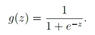
# Sigmoid function 激活函数
def sigmoid(z):
    return 1 / (1 + np.exp(-z))
-
cost(theta, X, y):计算损失
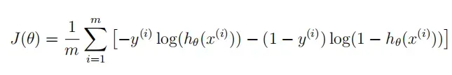
# Cost of logistic regression 计算logistic回归的损失函数 def cost(theta, X, y): first = -y * np.log(sigmoid(X @ theta)) second = (1 - y) * np.log(1 - sigmoid(X @ theta)) return np.mean(first - second) -
gradient(theta, X, y):计算梯度
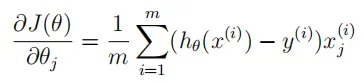
# Gradient of logistic regression 计算logistic回归的梯度 # The gradient of the cost is a vector of the same length as θ where the jth element (for j = 0, 1, . . . , n) def gradient(theta, X, y): return (X.T @ (sigmoid(X @ theta) - y)) / len(X) -
predict(theta, X):给定参数与数据集,做出预测
# Predict using parameters learned 利用学习的参数做出预测 # Return a list of predictions def predict(theta, X): probability = sigmoid(X @ theta) return [1 if x >= 0.5 else 0 for x in probability] -
featureMapping(x1, x2, power):特征映射
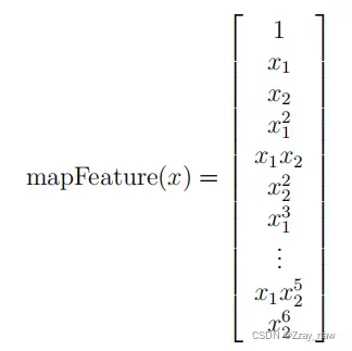
# Feature mapping 特征映射
def featureMapping(x1, x2, power):
    data = {}
    for i in np.arange(power + 1):
        for p in np.arange(i + 1):
            data["f{}{}".format(i - p, p)] = np.power(x1, i - p) * np.power(x2, p)
    return pd.DataFrame(data)
-
costReg(theta, X, y, l=1):正规化logistic回归的损失函数
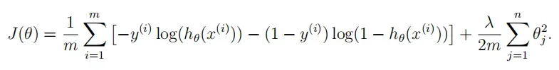
注意要特殊处理 θ0。
# Cost of regularize logistic regression function 计算正规化logistic回归函数的损失 def costReg(theta, X, y, l=1): theta_penalty = theta[1:] origin = cost(theta, X, y) addition = (l * theta_penalty @ theta_penalty) / (2 * len(X)) return origin + addition -
gradientReg(theta, X, y, l=1):正规化logistic回归的梯度计算
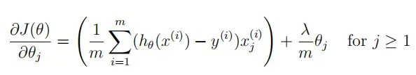
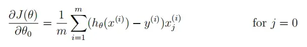
注意要特殊处理 θ0。
# Gradient of regularized logistic regression 计算正规化logistic回归的梯度
def gradientReg(theta, X, y, l=1):
    addition = l * theta / len(X)
    addition[0] = 0
    return gradient(theta, X, y) + addition
1. Logistic Regression
Implement the logstic regression.
- 需要特别注意
np.array()和np.asmatrix()的区别和应用场景。- 调用的相关函数在文章头部”Self-created functions”中详细描述。
# 1. Logistic Regression

path_data1 = '../data/ex2data1.txt'
df1 = pd.read_csv(path_data1, names=['Exam1', 'Exam2', 'Admitted'])
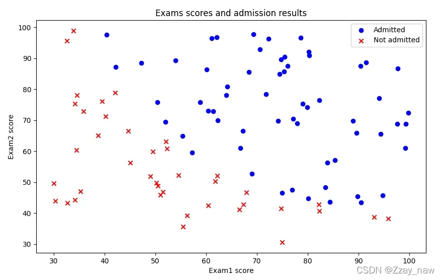
1.1 Visualization
# 1.1 Visualizing the data

# Separate the admitted students and the other
positive = df1[df1['Admitted'].isin(['1'])]
negative = df1[df1['Admitted'].isin(['0'])]

# Plot the figure
fig, fig_data = plt.subplots(figsize=[10, 6])
fig_data.scatter(positive['Exam1'], positive['Exam2'], c='b', label='Admitted')
fig_data.scatter(negative['Exam1'], negative['Exam2'], c='r', label='Not admitted', marker='x')
fig_data.legend(loc=1)
fig_data.set_xlabel('Exam1 score')
fig_data.set_ylabel('Exam2 score')
fig_data.set_title('Exams scores and admission results')
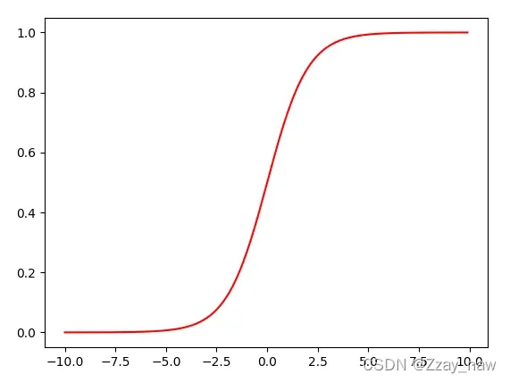
1.2 Sigmoid function
# 1.2 Implementation

# 1.2.1 Sigmoid function 激活函数
print(func.sigmoid(0))
x1 = np.arange(-10, 10, 0.1)
plt.plot(x1, func.sigmoid(x1), c='r')
1.3 Cost function & Gradient
# 1.2.2 Cost function and gradient 损失函数和梯度计算
if 'ONES' not in df1.columns:
    df1.insert(0, 'ONES', 1)
row = df1.shape[1]
X = np.array(df1.iloc[:, : -1])  # 注意这里使用np.array而不是np.matrix
y = np.array(df1.iloc[:, -1])
theta = np.zeros(X.shape[1])
print(func.cost(X, y, theta))
print(func.gradient(X, y, theta))
1.4 Learning θ using “fminunc”
源于Octave的fminunc函数是用来优化函数来计算成本和梯度参数。在Python中,我们可以用SciPy的optimize命名空间实现同样的操作。
此处我们调用的是高级优化算法,运行速度通常远远超过梯度下降。方便快捷。我们只需传入损失函数cost,参数θ,和梯度函数gradient。注意,cost函数的参数定义中θ需要为第一个;若cost函数只返回损失,则设置fprime=gradient。
这里使用fimin_tnc或者minimize方法来拟合,minimize中method可以选择不同的算法来计算,其中包括TNC。
# 1.2.3 Learning parameters using "fminunc" 通过优化函数学习参数
import scipy.optimize as opt

# opt.fmin_tnc()
res1 = opt.fmin_tnc(func=func.cost, x0=theta, args=(X, y), fprime=func.gradient)
print(res1)
# opt.minimize()
res2 = opt.minimize(fun=func.cost, x0=theta, args=(X, y), method='TNC', jac=func.gradient)
print(res2)

print(func.cost(res1[0], X, y))
print(func.cost(res2['x'], X, y))
以下是输出结果:
# opt.fmin_tnc()
(array([-25.1613186 ,   0.20623159,   0.20147149]), 36, 0)

# opt.minimize()
fun: 0.20349770158947475
     jac: array([8.86249424e-09, 7.33646598e-08, 4.72732538e-07])
 message: 'Local minimum reached (|pg| ~= 0)'
    nfev: 36
     nit: 17
  status: 0
 success: True
       x: array([-25.1613186 ,   0.20623159,   0.20147149])

# cost
0.20349770158947475
0.20349770158947475
1.5 Evaluation
编写一个函数,用我们所学的参数θ来为数据集X输出预测。然后,我们可以使用这个函数来给我们的分类器的训练精度打分。
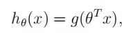
- logistic regression 模型的假设函数:
- 当
hθ大于等于 0.5 时,预测 y=1。 - 当
hθ小于 0.5 时,预测 y=0 。
- 当
# 1.2.4 Evaluating logistic regression
# 与原数据作对比检验
final_theta = res1[0]
predictions = func.predict(final_theta, X)
correct = [1 if a==b else 0 for (a, b) in zip(predictions, y)]
accuracy = sum(correct) / len(X)
print(accuracy)

# 利用sklearn包检验
from sklearn.metrics import classification_report
print(classification_report(predictions, y))
以下是输出结果:
0.89

              precision    recall  f1-score   support

           0       0.85      0.87      0.86        39
           1       0.92      0.90      0.91        61

    accuracy                           0.89       100
   macro avg       0.88      0.89      0.88       100
weighted avg       0.89      0.89      0.89       100
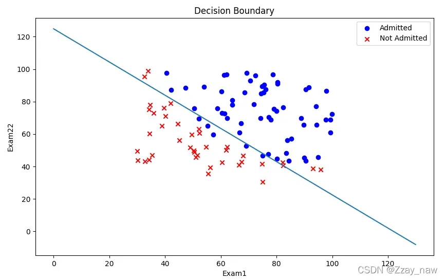
1.6 Decision Boundary
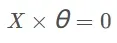
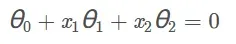
# 1.2.5 Decision Boundary
# ( theta[0] + theta[1] * x1 + theta[2] * x2 = 0 )
x1 = np.arange(130, step=0.1)
x2 = -(final_theta[0] + x1 * final_theta[1]) / final_theta[2]

# Visualization
fig, fig_bound = plt.subplots(figsize=(10, 6))
fig_bound.scatter(positive['Exam1'], positive['Exam2'], c='b', label='Admitted')
fig_bound.scatter(negative['Exam1'], negative['Exam2'], c='r', label='Not Admitted', marker='x')
fig_bound.plot(x1, x2)
fig_bound.legend(loc=1)
fig_bound.set_xlabel('Exam1')
fig_bound.set_ylabel('Exam22')
fig_bound.set_title('Decision Boundary')
plt.show()
2. Regularized logistic regression
In this section, we will optimize the logistic regression algorithm by regularization.
In short, regularization is a term in cost function that tilts algorithms toward simpler models that will carry smaller coefficients. This theory is helpful to reduce the occurrence of over-fitting and improve the generalization ability of the model.
- 需要特别注意
np.array()和np.asmatrix()的区别和应用场景。- 调用的相关函数在文章头部”Self-created functions”中详细描述。
# 2. Regularized logistic regression
path_data2 = '../data/ex2data2.txt'
df2 = pd.read_csv(path_data2, names=['Microchip Test 1', 'Microchip Test 2', 'Acceptance'])
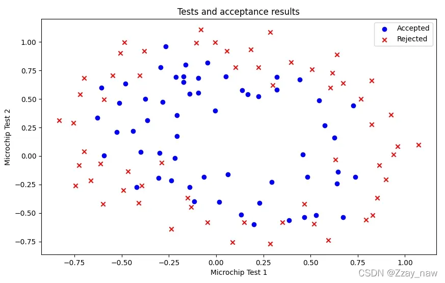
2.1 Visualization
# 2.1 Visualization
positive = df2[df2['Acceptance'].isin(['1'])]
negative = df2[df2['Acceptance'].isin(['0'])]

# Plot the figure
fig, fig_data2 = plt.subplots(figsize=[10, 6])
fig_data2.scatter(positive['Microchip Test 1'], positive['Microchip Test 2'], c='b', label='Accepted')
fig_data2.scatter(negative['Microchip Test 1'], negative['Microchip Test 2'], c='r', label='Rejected', marker='x')
fig_data2.legend(loc=1)
fig_data2.set_xlabel('Microchip Test 1')
fig_data2.set_ylabel('Microchip Test 2')
fig_data2.set_title('Tests and acceptance results')
plt.show()
2.2 Feature mapping
从上图可以注意到,其中的正负两类数据并没有线性的决策界限。因此,直接用 logistic回归在这个数据集上并不能表现良好,因为它只能用来寻找一个线性的决策边界。
一个拟合数据的更好的方法是从每个数据点创建更多的特征。我们将把这些特征映射到所有的x1和x2的多项式项上,直到第6次幂。
# 2.2 Feature Mapping
x1 = np.array(df2['Microchip Test 1'])
x2 = np.array(df2['Microchip Test 2'])
power = 6
regularized_data = func.featureMapping(x1, x2, power)
print(regularized_data)
2.3 Cost function & Gradient
# 2.3 Cost function and Gradient
X = regularized_data
y = np.array(df2['Acceptance'])
theta = np.zeros(X.shape[1])
print(func.costReg(theta, X, y, l=1))
print(func.gradientReg(theta, X, y, l=1))
2.4 Learning θ using “fminunc”
# 2.4 Learning parameters using "fminunc"
import scipy.optimize as opt

# Use opt.fmin_tnc()
res1 = opt.fmin_tnc(func=func.costReg, x0=theta, args=(X, y, 2), fprime=func.gradientReg)
print(res1)

# Use opt.minimize()
res2 = opt.minimize(fun=func.costReg, x0=theta, args=(X, y, 2), method='TNC', jac=func.gradientReg)
print(res2)

# Use "sklearn" lib
from sklearn import linear_model
model = linear_model.LogisticRegression(penalty='l2', C=1.0)
model.fit(X, y.ravel())
print(model.score(X, y))
以下为输出结果:
[res1]
(array([ 0.90267454,  0.33721089,  0.76006404, -1.39757946, -0.51417075,
       -0.91389985,  0.01516214, -0.21926017, -0.22677642, -0.16219637,
       -1.01270257, -0.04169398, -0.39984069, -0.14458017, -0.82296284,
       -0.20346048, -0.13186937, -0.04837714, -0.17183934, -0.17077936,
       -0.38820995, -0.72773035,  0.00607685, -0.19391899,  0.00314606,
       -0.21203169, -0.06947222, -0.69320886]), 25, 1)

[res2]
     fun: 0.5733984516596513
     jac: array([ 1.67633708e-06, -2.90856336e-06,  8.96406772e-07, -8.32612468e-07,
        1.02439563e-07,  1.90899668e-06, -1.35242750e-06, -3.59840239e-07,
       -1.69067486e-07,  1.29963371e-06, -2.18602082e-06, -3.80209746e-07,
       -8.12873068e-07, -9.17531075e-07,  6.41429367e-07, -9.19276291e-07,
        2.91038210e-07, -4.42204968e-07,  1.89624550e-07, -4.26240933e-07,
        1.14951260e-06, -1.69610321e-06,  4.20801504e-08,  4.32306883e-07,
        8.44834719e-08,  9.34045111e-08, -9.53173077e-08,  1.04936691e-06])
 message: 'Converged (|f_n-f_(n-1)| ~= 0)'
    nfev: 25
     nit: 6
  status: 1
 success: True
       x: array([ 0.90267454,  0.33721089,  0.76006404, -1.39757946, -0.51417075,
       -0.91389985,  0.01516214, -0.21926017, -0.22677642, -0.16219637,
       -1.01270257, -0.04169398, -0.39984069, -0.14458017, -0.82296284,
       -0.20346048, -0.13186937, -0.04837714, -0.17183934, -0.17077936,
       -0.38820995, -0.72773035,  0.00607685, -0.19391899,  0.00314606,
       -0.21203169, -0.06947222, -0.69320886])


0.8305084745762712
2.5 Evaluation
# 2.5 Evaluation
# 与原数据作对比检验
final_theta = res1[0]
predictions = func.predict(final_theta, X)
correct = [1 if a==b else 0 for (a, b) in zip(predictions, y)]
accuracy = sum(correct) / len(correct)
print(accuracy)

# Use "sklearn" lib
from sklearn.metrics import classification_report
print(classification_report(predictions, y))
以下为输出结果:
0.8305084745762712
              precision    recall  f1-score   support

           0       0.73      0.92      0.81        48
           1       0.93      0.77      0.84        70

    accuracy                           0.83       118
   macro avg       0.83      0.84      0.83       118
weighted avg       0.85      0.83      0.83       118
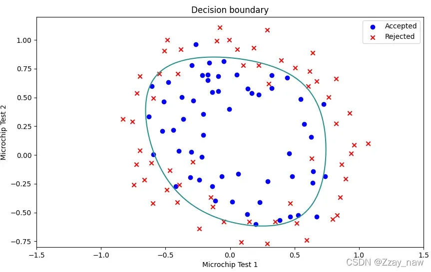
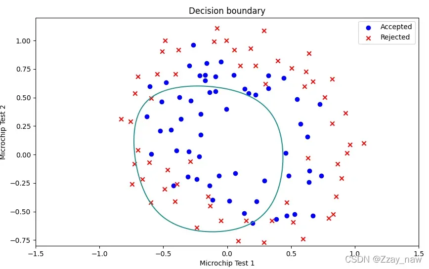
2.6 Decision boundary
# 2.6 Decision boundary
x = np.linspace(-1.5, 1.5, 250)
xx, yy = np.meshgrid(x, x)
z = np.asmatrix(func.featureMapping(xx.ravel(), yy.ravel(), 6))
z = z @ final_theta
z = z.reshape(xx.shape)

# Plot the figure
fig, fig_bound2 = plt.subplots(figsize=[10, 6])
fig_bound2.scatter(positive['Microchip Test 1'], positive['Microchip Test 2'], c='b', label='Accepted')
fig_bound2.scatter(negative['Microchip Test 1'], negative['Microchip Test 2'], c='r', label='Rejected', marker='x')
fig_bound2.legend(loc=1)
fig_bound2.set_xlabel('Microchip Test 1')
fig_bound2.set_ylabel('Microchip Test 2')
fig_bound2.set_title('Decision boundary')
plt.contour(xx, yy, z, 0)
plt.ylim(-0.8, 1.2)
plt.show()
- 当
λ == 1时:
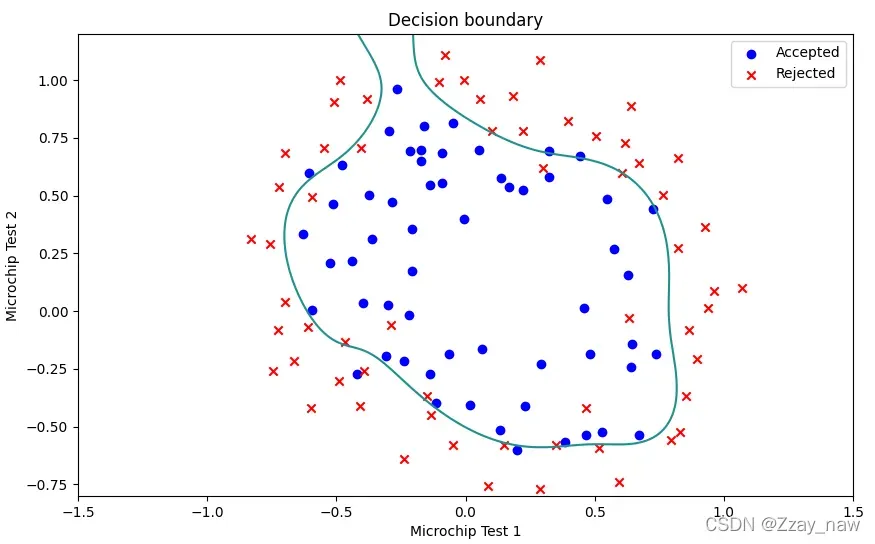
-
当
λ == 0时:出现**过拟合(overfitting)**现象。
-
当
λ == 100时:出现不准确的现象。
版权声明:本文为博主Zzay_naw原创文章,版权归属原作者,如果侵权,请联系我们删除!