Review:
2D Weight sparsity in DNNs
(Weight) Sparsity in Deep Learning_EverNoob的博客-CSDN博客
==> the above mentioned 2D sparsity is decidedly different from the 3D input sparsity scenario, in that we manually created the structured sparse weight to cut down memory footprint, while the 3D situation is caused by unstructured nature of point cloud or just the nature of high dimensionality;
====> the long and short of the unstructured sparse point cloud is: if we keep using dense operations, which the general purposed hardwares are poised to perform, we have to waste a LOT of time and energy on moving and computing 0s.
==> just check how we want the data to be structured for parallelled hardwares and how we exploited the structued sparsity for performance gains;
==> the main goal or method for 3D sparse convolution acceleration is hence to:
reduce memory footprint;
structurally format the sparsity (for efficient parallel processing)
Submanifold Sparse Convolutional Networks
the seminal paper that introduced the base method for currently popular sparse 3D convolution acceleration solutions:
https://arxiv.org/abs/1711.10275
[Submitted on 28 Nov 2017]
3D Semantic Segmentation with Submanifold Sparse Convolutional Networks
Benjamin Graham, Martin Engelcke, Laurens van der Maaten
Convolutional networks are the de-facto standard for analyzing spatio-temporal data such as images, videos, and 3D shapes. Whilst some of this data is naturally dense (e.g., photos), many other data sources are inherently sparse. Examples include 3D point clouds that were obtained using a LiDAR scanner or RGB-D camera. Standard “dense” implementations of convolutional networks are very inefficient when applied on such sparse data. We introduce new sparse convolutional operations that are designed to process spatially-sparse data more efficiently, and use them to develop spatially-sparse convolutional networks. We demonstrate the strong performance of the resulting models, called submanifold sparse convolutional networks (SSCNs), on two tasks involving semantic segmentation of 3D point clouds. In particular, our models outperform all prior state-of-the-art on the test set of a recent semantic segmentation competition.
key idea/purpose
One of the downsides of prior sparse implementations of convolutional networks is that they “dilate” the sparse data in every layer by applying “full” convolutions. In this work, we show that it is possible to create convolutional networks that keep the same level of sparsity throughout the network. To this end, we develop a new implementation for performing sparse convolutions (SCs) and introduce a novel convolution operator termed submanifold sparse convolution (SSC).1 We use these operators as the basis for submanifold sparse convolutional networks (SSCNs) that are optimized for efficient semantic segmentation of 3D point clouds
Definitions and Spatial Sparsity
We define a d-dimensional convolutional network as a network that takes as
input a (d + 1)-dimensional tensor: the input tensor contains d spatio-temporal dimensions (such as length, width, height, time, etc.) and one additional feature-space dimension (e.g., RGB color channels or surface normal vectors).
The input corresponds to a d-dimensional grid of sites, each of which is associated with a feature vector.
We define a site in the input to be active if any element in the feature vector is not in its ground state, e.g., if it is non-zero3.
In many problems, thresholding may be used to eliminate input sites at which the feature vector is within a small distance from the ground state.
Note that even though the input tensor is (d + 1)- dimensional, activity is a d-dimensional phenomenon: entire lines along the feature dimension are either active or inactive ==> e.g. a point either exists or not in point cloud, so, naturally, does its feature vector.
Similarly, the hidden layers of a d-dimensional convolutional network are represented by d-dimensional grids of feature-space vectors. a site in a hidden layer is active if any of the sites in the layer that it takes as input is active state.
The value of the ground state only needs to be calculated once per forward pass at training time, and only once for all forward passes at test time. This allows for substantial savings in computational and memory requirements; the exact savings depend on data sparsity and network depth.
“we argue that the framework described above is unduly restrictive”
Submanifold Dilation
If the input data contains a single active site, then after applying a 3d convolution, there will be 3d active sites. Applying a second convolution of the same size will yield 5d active sites, and so on. This rapid growth of the number of active sites is a poor prospect when implementing modern convolutional network architectures that comprise tens or even hundreds of convolutional layers, such as VGG networks, ResNets, or DenseNets [8, 9, 20].
Sparse Convolutional Networks and SSC
restricts the output of the convolution only to the set of active input points.
A potential problem of this approach is that hidden layers in the network may not receive all the information they require to classify the input data: in particular, two neighboring connected components are treated completely independently. We resolve this problem by using convolutional networks that incorporate some form of pooling, or use strided convolutions. Such operations are essential in the sparse convolutional networks4 we investigate, as they allow information to flow between disconnected components in the input. The closer the components are spatially, the fewer strided operations are necessary for the components to “communicate” in the intermediate representations.
SC
define a sparse convolution SC(m; n; f; s) with m input feature planes, n output feature planes, a filter size of f, and stride s. An SC convolution computes the set ofactive sites in the same way as a regular convolution: it looks for the presence of any active sites in its receptive
SSC
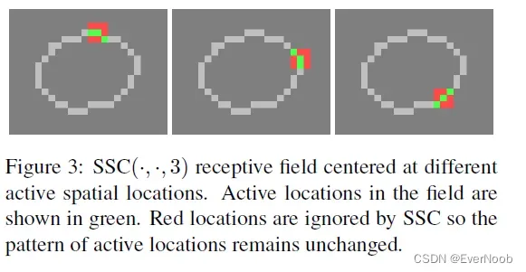
Let f denote an odd number. We define a submanifold sparse convolution SSC(m; n; f) as a modified SC(m; n; f; s = 1) convolution.
First, we pad the input with (f – 1)/2 zeros on each side (==> to keep input dimension)Next, we restrict an output site to be active if and only if the site at the corresponding site in the input is active (i.e., if the central site in the receptive field is active). ==> figure 3 above
Submanifold sparse convolutions are similar to Oct-Nets [18] in that they preserve the sparsity structure. However, unlike OctNets, empty space imposes no computational or memory overhead in the implementation of submanifold sparse convolutions.
==> naturally we have to restrict other necessary NN-operators, such as pooling, bn and activation to active sites accordingly.
the next section presents an article digesting the essentials of the SC/SSC’s implementation.
SpConv
https://towardsdatascience.com/how-does-sparse-convolution-work-3257a0a8fd1
==> the author for the quoted article is an ethnic Chinese living in Saxony, so just ignore the occassional grammar mistakes.
One intuitive thinking is, regular image signals are stored as matrix or tensor. And the corresponding convolution was calculated as dense matrix multiplication. The sparse signals are normally represented as data lists and index lists. We could develop a special convolution schema that uses the advantage of sparse signal representation.
3. Sparse Convolution Model
In a short, the traditional convolution uses FFT or im2col [5] to build the computational pipeline. Sparse Convolution collects all atomic operations w.r.t convolution kernel elements and saves them in a Rulebook as instructions of computation.
Below is an example, which explains how sparse convolution works.
3.1 Input Data Model
In order to explain the concept of sparse convolution step by step and let it easier to read, I use 2D sparse image processing as an example. Since the sparse signals are represented with data list and index list, 2D and 3D sparse signals have no essential difference.
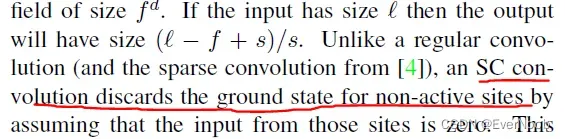
Fig.2 an example sparse image, all elements are zero except P1, P2. Image by Author
As Fig.2 illustrated, we have a 5×5 image with 3 channels. All the pixels are (0, 0, 0) except two points P1 and P2. P1 and P2, such nonzero elements are also called active input sites, according to [1]. In dense form, the input tensor has a shape [1x3x5x5] with NCHW order. In sparse form, the data list is
[[0.1, 0.1, 0.1], [0.2, 0.2, 0.2]], and the index list is[[1,2], [2, 3]]with YX order.3.2 Convolution Kernel
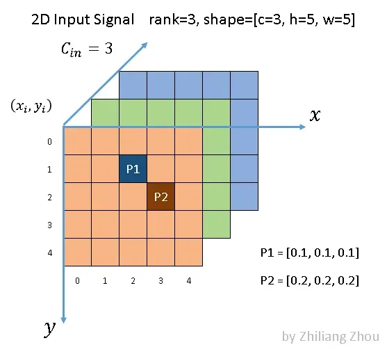
Fig.3 an example kernel. Image by Author
The convolution kernel of sparse convolution is the same as traditional convolution. Fig.3 is an example, which has kernel size 3×3. The dark and light colors stand for 2 filters. In this example, we use the following convolution parameters.
conv2D(kernel_size=3, out_channels=2, stride=1, padding=0)3.3 Output Definitions
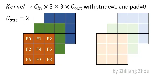
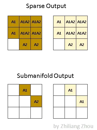
The output of the sparse convolution is quite different from traditional convolution. The sparse convolution has 2 kinds of output definitions [1]. One is regular output definition, just like ordinary convolution, calculate the output sites as long as kernel covers an input site. The other one is called the submanifold output definition. the convolution output will be counted only when the kernel center covers an input site. ==> dense allows any overlap, and we would enlarge the valued regions greatly, which is very often undesirable in both performance and accuracy
Fig.4 Two kinds of output definition. Image by Author
Fig.4 illustrates the difference between these two kinds of outputs. A1 stands for the active output sites, i.e. the convolution result from P1. Similarly, A2 stands for the active output sites which are calculated from P2. A1A2 stands for the active output sites which are the sum of outputs from P1 and P2. Dark and light colors stand for different output channels.
So in dense form, the output tensor has a shape [1x2x3x3] with NCHW order. In sparse form, the output has two lists, a data list, and an index list, which are similar to the input representation.
4. Computation Pipeline
Traditional convolution normally uses im2col [5] to rewrite convolution as a dense matrix multiplication problem. However, sparse convolution [1] uses a Rulebook to schedule all atomic operations instead of im2col.
4.1 Build the hash table
The first step is to build hash tables.
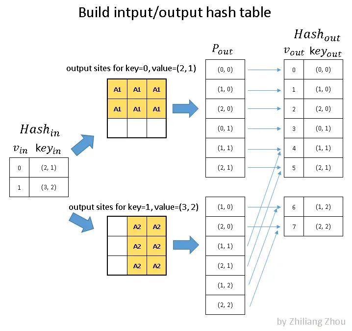
Fig.5 build hash tables for active input sites and active output sites. P_out is the position index. Image by Author
==> notation note:
==> “v” which is the key of the hashmap is just a uniquely valued list of index
==> “key” which is the value/item of the hashmap and records coordinates of the input sites, in XY-order; recall from part 3.1, the “index” list or the list of input site coordinates directly maps to data list hence we don’t need to include data at this step
In fig.5, the input hash table stores all active input sites. Then we estimated all possible active output sites, considering either regular output definition or submanifold output definition. At last, using the output hash table to record all involved active output sites.
4.2 Build Rule Book
The second step is to build the Rulebook. This is the key part of sparse convolution. The purpose of Rulebook is similar to im2col [5], which converts convolution from mathematic form to an efficient programmable form. But unlike im2col, Rulebook collects all involved atomic operation in convolution, then associate them to corresponding kernel elements.
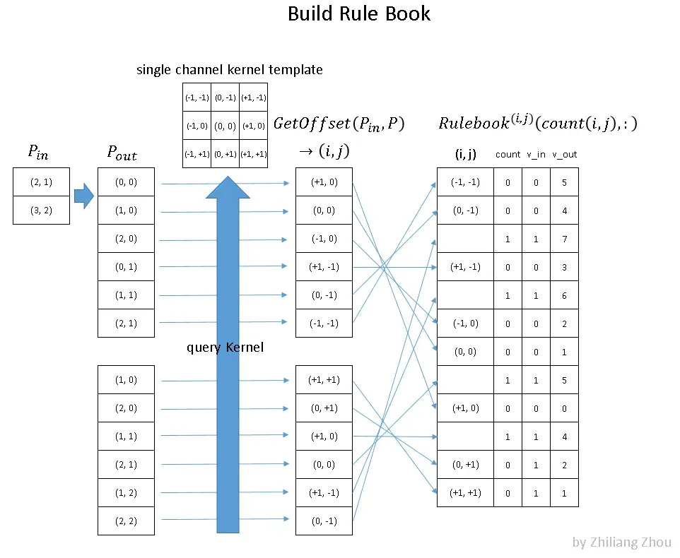
Fig.6 build rule book to schedule all atomic operations based on kernel index. Image by Author
Fig.6 is an example of how to build Rulebook. Pᵢₙ has the input sites index. In this example, we have two nonzero data at position (2, 1) and (3, 2). Pₒᵤₜ has the corresponding output sites index. Then we collect the atomic operations from the convolution calculation process, i.e. consider the convolution process as many atomic operations w.r.t kernel elements. At last, we record all atomic operations into Rulebook. In Fig.6 the right table is an example of the Rulebook. The first column is the kernel element index. ==> position by “offset” to the center of the kernel; The second column is a counter and index about how many atomic operations this kernel element involves. The third and fourth column is about the source and result of this atomic operation ==> by their indices from associated hashmap.
==> on “query Kernel” step:
===> use in(2,1), out(0,0) –> kernel(1,0) as an example:
for input site (2,1) to produce an output at (0,0) site of the convolution result (which is 3*3 in out setup), we know that the kernel must be applied at fm(1,1), i.e. x=1,y=1 at the feature map, and the kernel element at k(1,0) must be multiplied to the input site in(2,1) to produce out(0,0)
===> as we see in the graph above,
in(3,2), out(1,1) also involve kernel(1,0) and we append this entry to the rule book under the element index; differentiated from the previous one by count_index
===> the in/out position pair involves 1 and only 1 kernel element a time
4.3 Computation Pipeline for GPU
The last step is the overview of the programming calculation pipeline.
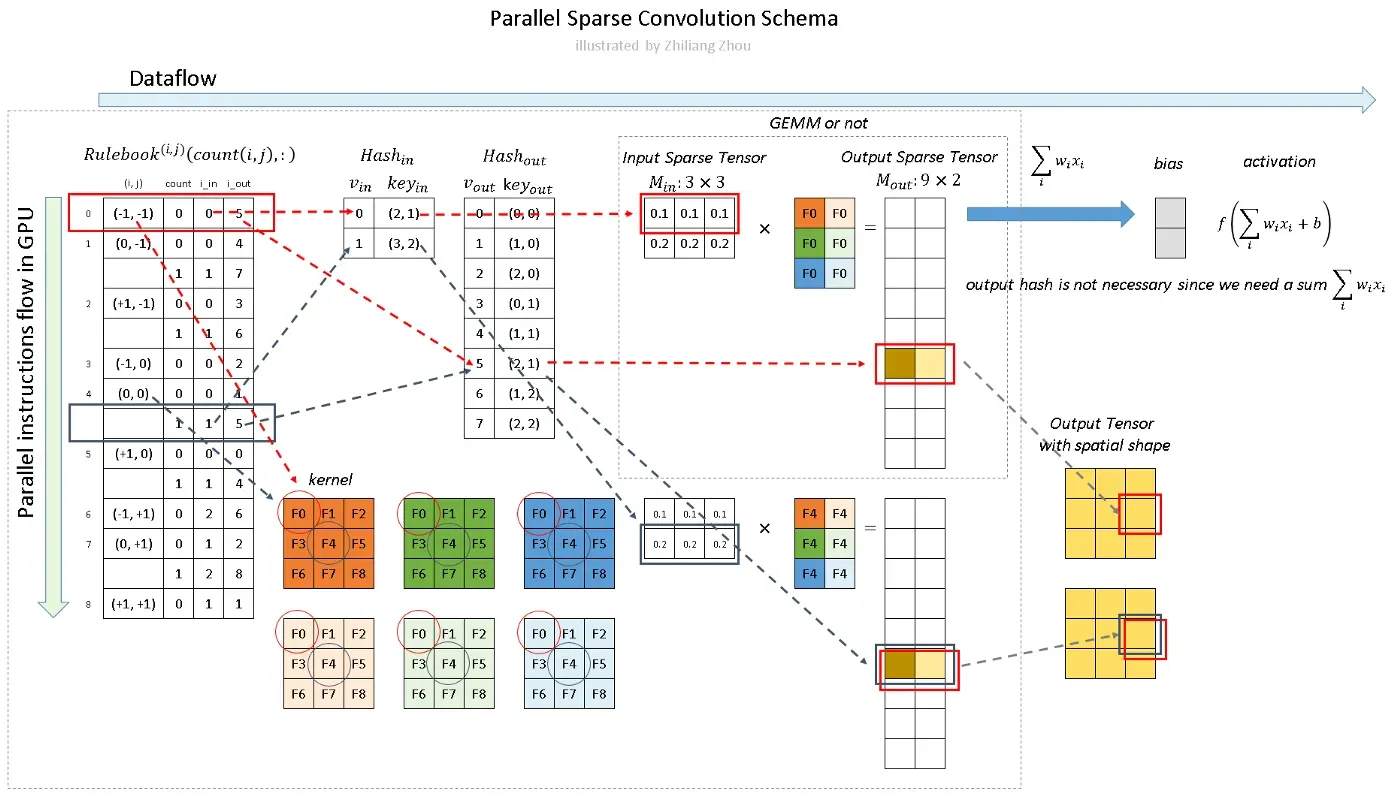
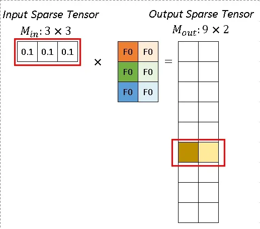
Fig.7 Calculation of sparse convolution. Image by Author
==> the “Output Tensor with spatial shape” is better presented as two 3*3 squares, brown for the first fitler’s result and light yellow for the second filter’s.
As Fig.7 illustrates, we calculate the convolution, not like the sliding window approach but calculate all the atomic operations according to Rulebook. In Fig.7 red and blue arrows indicate two examples.
In Fig.7 red and blue arrows indicate two calculation instances. The red arrow processes the first atomic operation for kernel element (-1, -1). From Rulebook, we know this atomic operation has input from P1 with position (2, 1) and has output with position (2, 1). This entire atomic operation can be constructed as Fig. 8.
Fig. 8 Atomic Operation. Image by Author
Similarly, the blue arrow indicates another atomic operation, which shares the same output site. The result from the red arrow instance and the blue arrow instance can be added together.
However, in practice, the neural network calculates the sum of the linear transformation with activation function like f(∑ wᵢ xᵢ +b). So we don’t really need the hash table for active output sites, just sum all of the atomic operation results together.
The computation w.r.t the Rulebook can be parallel launched in GPU.
5. Conclusion and Summary
So the sparse convolution is quite efficient because we do not need to scan all the pixels or spatial voxels. We only calculate convolution for the nonzero elements. We use Rulebook instead of im2col to rewrite the sparse convolution into a compact linear transformation problem, or we say a compact matrix multiplication problem. One additional computation cost is building the Rulebook. Fortunately, this building work can be also parallel processed with GPU.
At last, I wrote a SpConv Lite library [4], which was derived from [2]. It was implemented by CUDA and packaged into a python library. I also made a real-time LiDAR object detector [6] based on SpConv Lite.
Minkowski CNN and MinkowskiEngine
this paper: https://arxiv.org/abs/1904.08755
introduced Minkowski CNN and the open source library Minkowskil Engine, whose documentations are linked below:
Welcome to MinkowskiEngine’s documentation! — MinkowskiEngine 0.5.3 documentation
the paper mainly dealt with 3D videos, but subsequent works used Minkowski Convolution, suitable for generalized sparse tensor convolution, in point cloud, due to the shared sparse nature.
so focus on the Minkowski Convolution and how it deals with unstructured sparsity.
In section 3 of the paper:
Sparse Tensor and [Minkowski] Convolution
A Chinese breakdown of the method can be found here: 点云中的Minkowski卷积 – 知乎
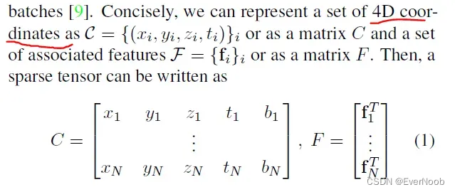
In traditional speech, text, or image data, features are extracted densely. Thus, the most common representations of these data are vectors, matrices, and tensors. However, for 3-dimensional scans or even higher-dimensional spaces, such dense representations are inefficient due to the sparsity. Instead, we can only save the non-empty part of the space as its coordinates and the associated features. This representation is an N-dimensional extension of a sparse matrix; thus it is known as a sparse tensor. There are many ways to save such sparse tensors compactly [31], but we follow the COO format as it is efficient for neighborhood queries (Sec. 3.1). Unlike the traditional sparse tensors, we augment the sparse tensor coordinates with the batch indices to distinguish points that occupy the same coordinate in different batches [9].
where bi and fi are the batch index and the feature associated to the i-th coordinate. In Sec. 6, we augment the 4D space with the 3D chromatic space and create a 7D sparse tensor for trilateral filtering.
==> from the breakdown:
D_f = len(f_i)
这样的表示,相比于[dense]3D卷积(X, Y, Z, D_f)的表示,可以节省空间。[N << XYZ -> N * 4 + N*D_f << XYZD_f, << 表示远小于]
3.1. Generalized Sparse Convolution
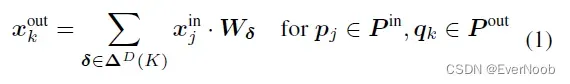
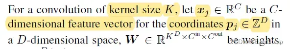
In this section, we generalize the sparse convolution [8, 9] for generic input and output coordinates and for arbitrary kernel shapes. The generalized sparse convolution encompasses not only all sparse convolutions but also the conventional dense convolutions.
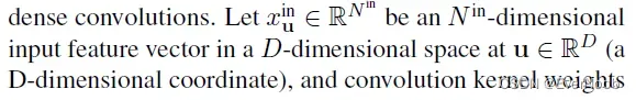
==> D here is strictly the dimension of coordinates, not related to feature;
==>recall
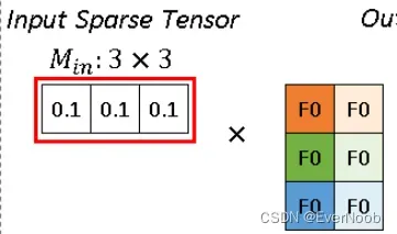
==> obviously, D_f = len(f_i) = N_in is the number of input “channels”, while N_out is the number of filters;
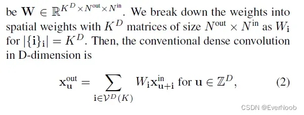
==> K is the kernel size, with D being the dimension of the convolutional space, and each weight matrix W_i corresponds to an “expanded” kernel element.
==> Right now, by this dense representation, we take every input x_u^in, mult to every kernel element W_i, and get every output x_u^out. We see in later generalized expression, we only need to choose valid input sites and the i/o pair associated kernel element.
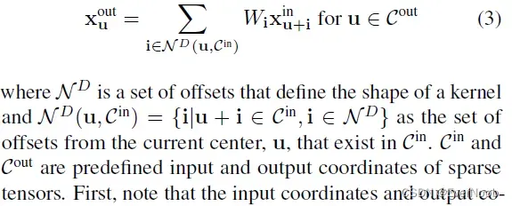
The generalized sparse convolution in Eq. 3 relaxes Eq. 2.
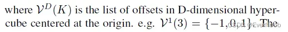
First, note that the input coordinates and output coordinates are not necessarily the same. Second, we define the shape of the convolution kernel arbitrarily with
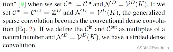
. This generalization encompasses many special cases such as the dilated convolution and typical hypercubic kernels. Another interesting special case is the “sparse submanifold convolution” [9]
==> C^out = C^in says that the sparsity is guaranteed to not dilate, which is the key idea/property of SSC;
====> pos(x_in) = stride * (x_out) + offset
SSC requires central match, hence offset = 0; when not using unit stride step, C^out <= C^in should suffice
==> by crafting the i/o site hashmap (C) and the RuleBook (N) we can have various forms of SC, such as full output version covered in the section above.
side note:
naming clearly adapted from https://en.wikipedia.org/wiki/Minkowski_space after Hermann Minkowski
Minkowski space (or Minkowski spacetime) (/mɪŋˈkɔːfski, -ˈkɒf-/[1]) is a combination of three-dimensional Euclidean space and time into a four-dimensional manifold where the spacetime interval between any two events is independent of the inertial frame of reference in which they are recorded. ==> yep, the man is Einstein’s own physics professor.
==> so the Minkowski part is really the introduction of time augmentation to form a 4D spatial-temporal space for convolution
TorchSparse: GPU based Point Cloud Inference SC Acceleration
TorchSparse: Efficient Point Cloud Inference Engine
Notation:
Mapping
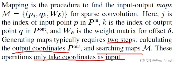
to get output position set:
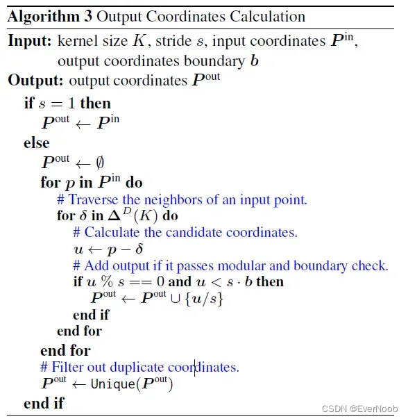
when down-sampling, since we want to sample as many sparse input sites as possible, we slack the SSC i/o mapping condition to p < s*b + offset, where:
==> instead of offset = 0, we check all possible offset for p to be matched to any kernel within output boundary, b_i <= B = (range(D_i) – s_i) / s_i + 1
====> u % s enforces kernel central matching after dilation
文章出处登录后可见!