Unet网络:利用DoubleConv, Down, Up, OutConv四个模块组装U-net模型,其中Up即右侧模型块之间的上采样连接(Up sampling)部分,注意U-net的跳跃连接(Skip-connection)也在这部分(torch.cat([x2, x1], dim=1))。因为每个子块内部的两次卷积(Double Convolution),所以上采样后也有DoubleConv层。
PyTorch模型定义的方式
1.Module类是torch.nn模块里提供的一个模型构造类 (nn.Module),是所有神经网络模块的基类,可以继承它来定义我们想要的模型;
2.Sequential,ModuleList和ModuleDict三种方式
PyTorch模型定义应包括两个主要部分:
(1)各个部分的初始化(init);
(2)数据流向定义(forward)
Sequential
1.nn.Sequential()即一个时序容器,Modules会以它们传入的顺序被添加到容器中。当模型的前向计算为简单串联各个层的计算时,Sequential类可以通过更加简单的方式定义模型。
2.它可以接收一个子模块的有序字典(OrderedDict)或者一系列子模块作为参数来逐一添加 Module 的实例,而模型的前向计算就是将这些实例按添加的顺序逐⼀计算。
3.使用Sequential定义模型的好处在于简单、易读,同时使用Sequential定义的模型不需要再写forward,因为顺序已经定义好了。但使用Sequential也会使得模型定义丧失灵活性,比如需要在模型中间加入一个外部输入时就不适合用Sequential的方式实现。使用时需根据实际需求加以选择。
结合Sequential和定义方式加以理解:
class MySequential(nn.Module):
    from collections import OrderedDict
    def __init__(self, *args):
        super(MySequential, self).__init__()
        if len(args) == 1 and isinstance(args[0], OrderedDict): # 如果传入的是一个OrderedDict
            for key, module in args[0].items():
                self.add_module(key, module)  # add_module方法会将module添加进self._modules(一个OrderedDict)
        else:  # 传入的是一些Module
            for idx, module in enumerate(args):
                self.add_module(str(idx), module)
    def forward(self, input):
        # self._modules返回一个 OrderedDict,保证会按照成员添加时的顺序遍历成
        for module in self._modules.values():
            input = module(input)
        return input
如何使用Sequential定义模型。您只需要按顺序排列模型的图层即可。根据层名的不同,有两种排列方式:
import torch.nn as nn
net = nn.Sequential(
        nn.Linear(784, 256),
        nn.ReLU(),
        nn.Linear(256, 10),
        )
print(net)

# 结果:
Sequential(
  (0): Linear(in_features=784, out_features=256, bias=True)
  (1): ReLU()
  (2): Linear(in_features=256, out_features=10, bias=True)
)
使用OrderedDict:
import collections
import torch.nn as nn
net2 = nn.Sequential(collections.OrderedDict([
          ('fc1', nn.Linear(784, 256)),
          ('relu1', nn.ReLU()),
          ('fc2', nn.Linear(256, 10))
          ]))
print(net2)

# 结果:
Sequential(
  (fc1): Linear(in_features=784, out_features=256, bias=True)
  (relu1): ReLU()
  (fc2): Linear(in_features=256, out_features=10, bias=True)
)
ModuleList
对应的模块是nn.ModuleList()。
ModuleList 接收一个子模块(或层,需属于nn.Module类)的列表作为输入,然后也可以类似List那样进行append和extend操作。
子模块或层的权重也会自动添加到网络中。
net = nn.ModuleList([nn.Linear(784, 256), nn.ReLU()])
net.append(nn.Linear(256, 10)) # # 类似List的append操作
print(net[-1])  # 类似List的索引访问
print(net)

# 结果为:
Linear(in_features=256, out_features=10, bias=True)
ModuleList(
  (0): Linear(in_features=784, out_features=256, bias=True)
  (1): ReLU()
  (2): Linear(in_features=256, out_features=10, bias=True)
)
注意:nn.ModuleList并没有定义一个网络,它只是将不同的模块储存在一起。ModuleList中元素的先后顺序并不代表其在网络中的真实位置顺序,需要经过forward函数指定各个层的先后顺序后才算完成了模型的定义。具体实现时用for循环即可完成:
class model(nn.Module):
  def __init__(self, ...):
    self.modulelist = ...
    ...

  def forward(self, x):
    for layer in self.modulelist:
      x = layer(x)
    return x
ModuleDict
对应模块为nn.ModuleDict(),从名字也看出是一个字典,ModuleDict和ModuleList的作用类似,只是ModuleDict能够更方便地为神经网络的层添加名称(value),并且访问时可以直接用key值引用。
net = nn.ModuleDict({
    'linear': nn.Linear(784, 256),
    'act': nn.ReLU(),
})
net['output'] = nn.Linear(256, 10) # 添加
print(net['linear']) # 访问
print(net.output)
print(net)

# 结果为
Linear(in_features=784, out_features=256, bias=True)
Linear(in_features=256, out_features=10, bias=True)
ModuleDict(
  (act): ReLU()
  (linear): Linear(in_features=784, out_features=256, bias=True)
  (output): Linear(in_features=256, out_features=10, bias=True)
)
三种方式的比较及适用场景
Sequential适合快速验证结果,因为已经明确了要用哪些层,直接写就行了,不用同时写__init__和forward;ModuleList和ModuleDict在某个完全相同的层需要重复出现多次时,非常方便实现,可以”一行顶多行“;当我们需要之前层的信息的时候,比如 ResNets 中的 残差计算,当前层的结果需要和之前层中的结果进行融合,一般使用 ModuleList/ModuleDict 比较方便。
U-Net
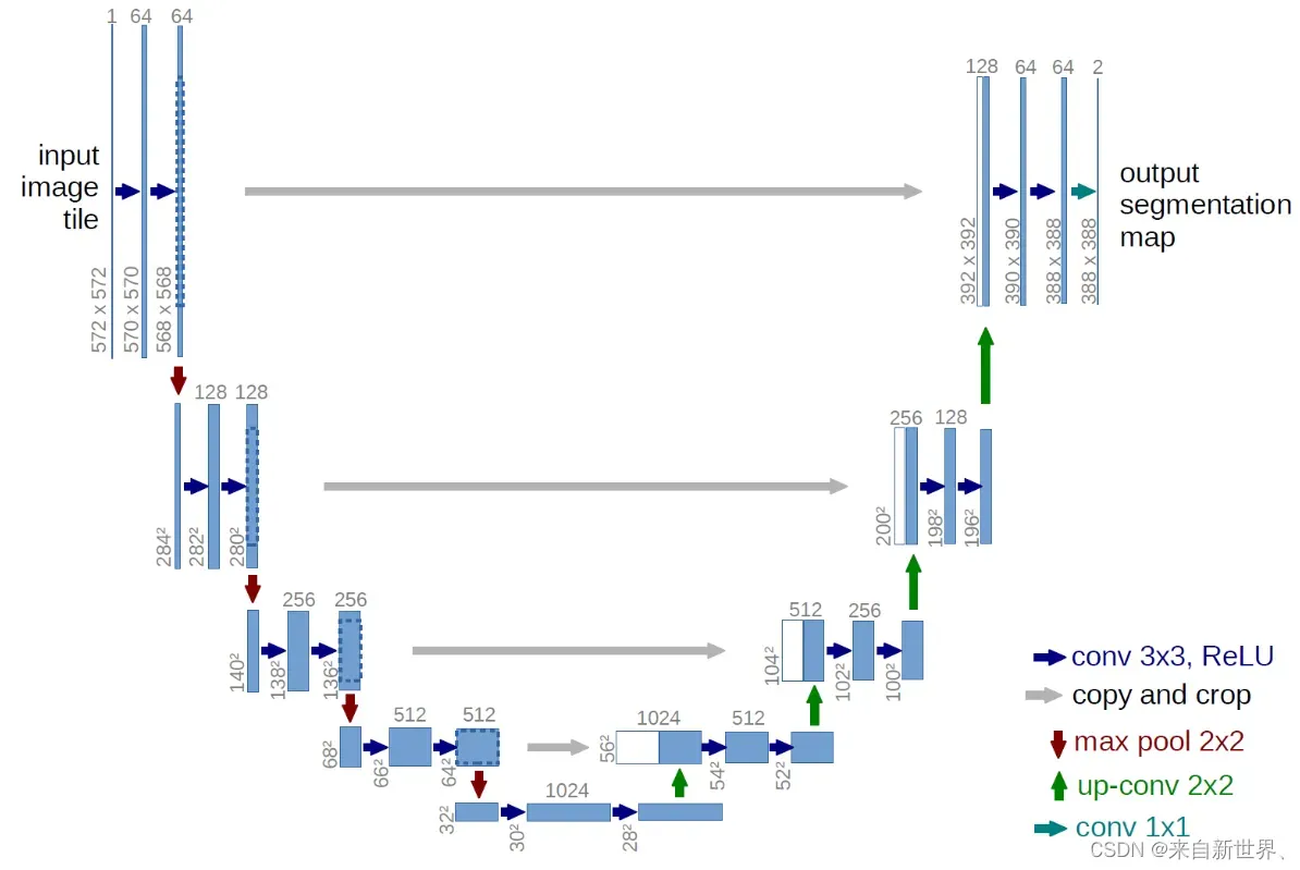
U-Net模型块分析
U-Net模型具有非常好的对称性。由于模型的形状非常像英文字母的“U”,因此被命名为“U-Net”。
模型从上到下分为几层,每层由左右两个模型块组成,每侧的模型块与上下模型块相连;
同时位于同一层左右两侧的模型块之间也有连接,称为“Skip-connection”。
还有其他组件,例如输入和输出处理。
组成U-Net的模型块主要有如下几个部分:
1.每个子块内部的两次卷积(Double Convolution)
2.左侧模型块之间的下采样连接,通过Max pooling来实现
3.右侧模型块之间的上采样连接(Up sampling)
输出层的处理
4.除模型块外,还有模型块之间的横向连接,输入和U-Net底部的连接等计算,这些单独的操作可以通过forward函数来实现。
除模型块外,还有模型块之间的横向连接,输入和U-Net底部的连接等计算,这些单独的操作可以通过forward函数来实现。
U-Net模型块实现
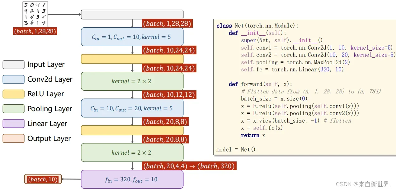
DoubleConv即每个子块内部的两次卷积(Double Convolution)。
这里回顾下CNN卷积神经网络,我们可以很方便地使用nn.Con2d层,
并且注意一开始的input维度为batch_size, in_channels, width, height,
而Conv2d()的参数依次为输入通道数、输出通道数和kernel_size:
class DoubleConv(nn.Module):
    """(convolution => [BN] => ReLU) * 2"""

    def __init__(self, in_channels, out_channels, mid_channels=None):
        super().__init__()
        if not mid_channels:
            mid_channels = out_channels
        self.double_conv = nn.Sequential(
            nn.Conv2d(in_channels, mid_channels, kernel_size=3, padding=1, bias=False),
            nn.BatchNorm2d(mid_channels),
            nn.ReLU(inplace=True),
            nn.Conv2d(mid_channels, out_channels, kernel_size=3, padding=1, bias=False),
            nn.BatchNorm2d(out_channels),
            nn.ReLU(inplace=True)
        )

    def forward(self, x):
        return self.double_conv(x)
Down即左侧模型块之间的下采样连接,通过Max pooling来实现。因为每个子块内部的两次卷积(Double Convolution),所以最大池化后也有DoubleConv层。
class Down(nn.Module):
    """Downscaling with maxpool then double conv"""

    def __init__(self, in_channels, out_channels):
        super().__init__()
        self.maxpool_conv = nn.Sequential(
            nn.MaxPool2d(2),
            DoubleConv(in_channels, out_channels)
        )

    def forward(self, x):
        return self.maxpool_conv(x)
Up即右侧模型块之间的上采样连接(Up sampling)部分,
注意U-net的跳跃连接(Skip-connection)也在这部分(torch.cat([x2, x1], dim=1))。
因为每个子块内部的两次卷积(Double Convolution),所以上采样后也有DoubleConv层。
class Up(nn.Module):
    """Upscaling then double conv"""

    def __init__(self, in_channels, out_channels, bilinear=True):
        super().__init__()

        # if bilinear, use the normal convolutions to reduce the number of channels
        if bilinear:
            self.up = nn.Upsample(scale_factor=2, mode='bilinear', align_corners=True)
            self.conv = DoubleConv(in_channels, out_channels, in_channels // 2)
        else:
            self.up = nn.ConvTranspose2d(in_channels, in_channels // 2, kernel_size=2, stride=2)
            self.conv = DoubleConv(in_channels, out_channels)

    def forward(self, x1, x2):
        x1 = self.up(x1)
        # input is CHW
        diffY = x2.size()[2] - x1.size()[2]
        diffX = x2.size()[3] - x1.size()[3]

        x1 = F.pad(x1, [diffX // 2, diffX - diffX // 2,
                        diffY // 2, diffY - diffY // 2])
        # if you have padding issues, see
        # https://github.com/HaiyongJiang/U-Net-Pytorch-Unstructured-Buggy/commit/0e854509c2cea854e247a9c615f175f76fbb2e3a
        # https://github.com/xiaopeng-liao/Pytorch-UNet/commit/8ebac70e633bac59fc22bb5195e513d5832fb3bd
        x = torch.cat([x2, x1], dim=1)
        return self.conv(x)
class OutConv(nn.Module):
    def __init__(self, in_channels, out_channels):
        super(OutConv, self).__init__()
        self.conv = nn.Conv2d(in_channels, out_channels, kernel_size=1)

    def forward(self, x):
        return self.conv(x)
class OutConv(nn.Module):
    def __init__(self, in_channels, out_channels):
        super(OutConv, self).__init__()
        self.conv = nn.Conv2d(in_channels, out_channels, kernel_size=1)

    def forward(self, x):
        return self.conv(x)
利用模型块组装U-Net
class UNet(nn.Module):
    def __init__(self, n_channels, n_classes, bilinear=True):
        super(UNet, self).__init__()
        self.n_channels = n_channels
        self.n_classes = n_classes
        self.bilinear = bilinear

        self.inc = DoubleConv(n_channels, 64)
        self.down1 = Down(64, 128)
        self.down2 = Down(128, 256)
        self.down3 = Down(256, 512)
        factor = 2 if bilinear else 1
        self.down4 = Down(512, 1024 // factor)
        self.up1 = Up(1024, 512 // factor, bilinear)
        self.up2 = Up(512, 256 // factor, bilinear)
        self.up3 = Up(256, 128 // factor, bilinear)
        self.up4 = Up(128, 64, bilinear)
        self.outc = OutConv(64, n_classes)

    def forward(self, x):
        x1 = self.inc(x)
        x2 = self.down1(x1)
        x3 = self.down2(x2)
        x4 = self.down3(x3)
        x5 = self.down4(x4)
        x = self.up1(x5, x4)
        x = self.up2(x, x3)
        x = self.up3(x, x2)
        x = self.up4(x, x1)
        logits = self.outc(x)
        return logits
net = UNet(1, 10)
print(net)
这里我们定义随机输入数据,看通过模型后得到的维度,
注意下面的两个3的维度要对应,
第一个3是输入数据的input_channel(如彩色图像,就是RGB的三维channel),
第二个3是卷积层中传入的input_channel实参。
另外在我们randn的第一个参数是batch_size,即一次处理的样本数。
if __name__ == '__main__':
    # 输入为大小为256*256的RGB数据
    input_data = torch.randn(1, 3, 256, 256)
    print('输入的数据:\n',input_data.shape)
    net = UNet(3, 1)
    print('输出的数据维度:\n', net(input_data).shape)
    # print(summary(net, input_data.shape))
=======================================
输入的数据:
 torch.Size([1, 3, 256, 256])
输出的数据维度:
 torch.Size([1, 1, 256, 256])
通过pip install -i https://pypi.tuna.tsinghua.edu.cn/simple torchsummary我们可以使用torchsummary工具更好看清模型结构:
----------------------------------------------------------------
        Layer (type)               Output Shape         Param #
================================================================
            Conv2d-1         [-1, 64, 256, 256]           1,728
       BatchNorm2d-2         [-1, 64, 256, 256]             128
              ReLU-3         [-1, 64, 256, 256]               0
            Conv2d-4         [-1, 64, 256, 256]          36,864
       BatchNorm2d-5         [-1, 64, 256, 256]             128
              ReLU-6         [-1, 64, 256, 256]               0
        DoubleConv-7         [-1, 64, 256, 256]               0
         MaxPool2d-8         [-1, 64, 128, 128]               0
            Conv2d-9        [-1, 128, 128, 128]          73,728
      BatchNorm2d-10        [-1, 128, 128, 128]             256
             ReLU-11        [-1, 128, 128, 128]               0
           Conv2d-12        [-1, 128, 128, 128]         147,456
      BatchNorm2d-13        [-1, 128, 128, 128]             256
             ReLU-14        [-1, 128, 128, 128]               0
       DoubleConv-15        [-1, 128, 128, 128]               0
             Down-16        [-1, 128, 128, 128]               0
        MaxPool2d-17          [-1, 128, 64, 64]               0
           Conv2d-18          [-1, 256, 64, 64]         294,912
      BatchNorm2d-19          [-1, 256, 64, 64]             512
             ReLU-20          [-1, 256, 64, 64]               0
           Conv2d-21          [-1, 256, 64, 64]         589,824
      BatchNorm2d-22          [-1, 256, 64, 64]             512
             ReLU-23          [-1, 256, 64, 64]               0
       DoubleConv-24          [-1, 256, 64, 64]               0
             Down-25          [-1, 256, 64, 64]               0
        MaxPool2d-26          [-1, 256, 32, 32]               0
           Conv2d-27          [-1, 512, 32, 32]       1,179,648
      BatchNorm2d-28          [-1, 512, 32, 32]           1,024
             ReLU-29          [-1, 512, 32, 32]               0
           Conv2d-30          [-1, 512, 32, 32]       2,359,296
      BatchNorm2d-31          [-1, 512, 32, 32]           1,024
             ReLU-32          [-1, 512, 32, 32]               0
       DoubleConv-33          [-1, 512, 32, 32]               0
             Down-34          [-1, 512, 32, 32]               0
        MaxPool2d-35          [-1, 512, 16, 16]               0
           Conv2d-36          [-1, 512, 16, 16]       2,359,296
      BatchNorm2d-37          [-1, 512, 16, 16]           1,024
             ReLU-38          [-1, 512, 16, 16]               0
           Conv2d-39          [-1, 512, 16, 16]       2,359,296
      BatchNorm2d-40          [-1, 512, 16, 16]           1,024
             ReLU-41          [-1, 512, 16, 16]               0
       DoubleConv-42          [-1, 512, 16, 16]               0
             Down-43          [-1, 512, 16, 16]               0
         Upsample-44          [-1, 512, 32, 32]               0
           Conv2d-45          [-1, 512, 32, 32]       4,718,592
      BatchNorm2d-46          [-1, 512, 32, 32]           1,024
             ReLU-47          [-1, 512, 32, 32]               0
           Conv2d-48          [-1, 256, 32, 32]       1,179,648
      BatchNorm2d-49          [-1, 256, 32, 32]             512
             ReLU-50          [-1, 256, 32, 32]               0
       DoubleConv-51          [-1, 256, 32, 32]               0
               Up-52          [-1, 256, 32, 32]               0
         Upsample-53          [-1, 256, 64, 64]               0
           Conv2d-54          [-1, 256, 64, 64]       1,179,648
      BatchNorm2d-55          [-1, 256, 64, 64]             512
             ReLU-56          [-1, 256, 64, 64]               0
           Conv2d-57          [-1, 128, 64, 64]         294,912
      BatchNorm2d-58          [-1, 128, 64, 64]             256
             ReLU-59          [-1, 128, 64, 64]               0
       DoubleConv-60          [-1, 128, 64, 64]               0
               Up-61          [-1, 128, 64, 64]               0
         Upsample-62        [-1, 128, 128, 128]               0
           Conv2d-63        [-1, 128, 128, 128]         294,912
      BatchNorm2d-64        [-1, 128, 128, 128]             256
             ReLU-65        [-1, 128, 128, 128]               0
           Conv2d-66         [-1, 64, 128, 128]          73,728
      BatchNorm2d-67         [-1, 64, 128, 128]             128
             ReLU-68         [-1, 64, 128, 128]               0
       DoubleConv-69         [-1, 64, 128, 128]               0
               Up-70         [-1, 64, 128, 128]               0
         Upsample-71         [-1, 64, 256, 256]               0
           Conv2d-72         [-1, 64, 256, 256]          73,728
      BatchNorm2d-73         [-1, 64, 256, 256]             128
             ReLU-74         [-1, 64, 256, 256]               0
           Conv2d-75         [-1, 64, 256, 256]          36,864
      BatchNorm2d-76         [-1, 64, 256, 256]             128
             ReLU-77         [-1, 64, 256, 256]               0
       DoubleConv-78         [-1, 64, 256, 256]               0
               Up-79         [-1, 64, 256, 256]               0
           Conv2d-80          [-1, 1, 256, 256]              65
          OutConv-81          [-1, 1, 256, 256]               0
================================================================
Total params: 17,262,977
Trainable params: 17,262,977
Non-trainable params: 0
----------------------------------------------------------------
Input size (MB): 0.75
Forward/backward pass size (MB): 942.00
Params size (MB): 65.85
Estimated Total Size (MB): 1008.60
----------------------------------------------------------------
None
PyTorch修改模型
如何在现有模型的基础上修改模型的几层
如何向现有模型添加额外的输入
如何向现有模型添加额外的输出
修改ResNet50模型层做10分类任务
import torchvision.models as models
net = models.resnet50()
print(net)
ResNet(
  (conv1): Conv2d(3, 64, kernel_size=(7, 7), stride=(2, 2), padding=(3, 3), bias=False)
  (bn1): BatchNorm2d(64, eps=1e-05, momentum=0.1, affine=True, track_running_stats=True)
  (relu): ReLU(inplace=True)
  (maxpool): MaxPool2d(kernel_size=3, stride=2, padding=1, dilation=1, ceil_mode=False)
  (layer1): Sequential(
    (0): Bottleneck(
      (conv1): Conv2d(64, 64, kernel_size=(1, 1), stride=(1, 1), bias=False)
      (bn1): BatchNorm2d(64, eps=1e-05, momentum=0.1, affine=True, track_running_stats=True)
      (conv2): Conv2d(64, 64, kernel_size=(3, 3), stride=(1, 1), padding=(1, 1), bias=False)
      (bn2): BatchNorm2d(64, eps=1e-05, momentum=0.1, affine=True, track_running_stats=True)
      (conv3): Conv2d(64, 256, kernel_size=(1, 1), stride=(1, 1), bias=False)
      (bn3): BatchNorm2d(256, eps=1e-05, momentum=0.1, affine=True, track_running_stats=True)
      (relu): ReLU(inplace=True)
      (downsample): Sequential(
        (0): Conv2d(64, 256, kernel_size=(1, 1), stride=(1, 1), bias=False)
        (1): BatchNorm2d(256, eps=1e-05, momentum=0.1, affine=True, track_running_stats=True)
      )
    )
..............
  (avgpool): AdaptiveAvgPool2d(output_size=(1, 1))
  (fc): Linear(in_features=2048, out_features=1000, bias=True)
)
这里模型结构是为了适配ImageNet预训练的权重,因此最后全连接层(fc)的输出节点数是1000。
对原始模型进行两处修改:
假设我们要用这个resnet模型去做一个10分类的问题,就应该修改模型的fc层,将其输出节点数替换为10。
我们觉得一个全连接层可能太少了,想再加一层。
from collections import OrderedDict
classifier = nn.Sequential(OrderedDict([('fc1', nn.Linear(2048, 128)),
                          ('relu1', nn.ReLU()),
                          ('dropout1',nn.Dropout(0.5)),
                          ('fc2', nn.Linear(128, 10)),
                          ('output', nn.Softmax(dim=1))
                          ]))

net.fc = classifier
这里的操作相当于将模型(net)最后名称为“fc”的层替换成了我们自己定义的名称为“classifier”的结构。使用Sequential+OrderedDict的模型定义方式。现在的模型就可以去做10分类任务了。
添加外部输入
有时候在模型训练中,除了已有模型的输入之外,还需要输入额外的信息。比如在CNN网络中,我们除了输入图像,还需要同时输入图像对应的其他信息,这时候就需要在已有的CNN网络中添加额外的输入变量。
基本思路:将输入位置作为一个整体加入之前,取原始模型的一部分,同时在forward中定义好原模型不变的部分、添加的输入和后续层之间的连接关系,从而完成模型的修改。
我们以torchvision的resnet50模型为基础,任务还是10分类任务。
不同点在于,我们希望利用已有的模型结构,在倒数第二层增加一个额外的输入变量add_variable来辅助预测。具体实现如下:
import torch.nn as nn
import  torch
import torchvision.models as models
from collections import OrderedDict
# 添加外部输入
class Model(nn.Module):
    def __init__(self, net):
        super(Model, self).__init__()
        self.net = net
        self.relu = nn.ReLU()
        self.dropout = nn.Dropout(0.5)
        self.fc_add = nn.Linear(1001, 10, bias=True)
        self.output = nn.Softmax(dim=1)

    def forward(self, x, add_variable):
        # net(x)为resnet50()
        x = self.net(x)
        # 增加一个额外的输入变量add_variable,辅助预测
        # 添加 self.dropout(self.relu(x)) 的输出为1000维,add_variable.unsqueeze(1))为1维
        # cat之后1001维度
        x = torch.cat((self.dropout(self.relu(x)),
        			  add_variable.unsqueeze(1)),
        			  1)
        x = self.fc_add(x)
        x = self.output(x)
        return x

net = models.resnet50()
print('添加额外输入之前:\n', net)
model = Model(net)
print('添加额外输入之后:\n', model)
# 另外别忘了,训练中在输入数据的时候要给两个inputs:
# outputs = model(inputs, add_var)
这里的实现要点是通过torch.cat实现了tensor的拼接。torchvision中的resnet50输出是一个1000维的tensor,我们通过修改forward函数(配套定义一些层),先将2048维的tensor通过激活函数层和dropout层,再和外部输入变量”add_variable”拼接,之后再通过全连接层映射到指定的输出维度10。
另外这里对外部输入变量”add_variable”进行unsqueeze操作是为了和net输出的tensor保持维度一致,常用于add_variable是单一数值 (scalar) 的情况,此时add_variable的维度是 (batch_size),需要在第二维补充维数1,从而可以和tensor进行torch.cat操作。
实例化我们修改后的模型结构后,我们可以使用它:
import torchvision.models as models
net = models.resnet50()
model = Model(net).cuda()
另外别忘了,训练中在输入数据的时候要给两个inputs:
outputs = model(inputs, add_var)
添加额外的输出
有时在模型训练中,除了模型的最终输出,我们还需要输出模型的一个中间层的结果,以应用额外的监督,获得更好的中间层结果。
基本思想是在模型定义中修改forward函数的return变量。
依然以resnet50做10分类任务为例,在已经定义好的模型结构上,同时输出1000维的倒数第二层和10维的最后一层结果。
具体实现如下:
import torch.nn as nn
import  torch
import torchvision.models as models
from collections import OrderedDict

# 添加额外输出
class Model(nn.Module):
    def __init__(self, net):
        super(Model, self).__init__()
        self.net = net
        self.relu = nn.ReLU()
        self.dropout = nn.Dropout(0.5)
        self.fc1 = nn.Linear(1000, 10, bias=True)
        self.output = nn.Softmax(dim=1)

    def forward(self, x):
        x1000 = self.net(x)
        x10 = self.dropout(self.relu(x1000))
        x10 = self.fc1(x10)
        x10 = self.output(x10)
        # 输出倒数第二层x1000,和最后一层x10
        return x10, x1000

net = models.resnet50()
print('添加额外输出之前:\n', net)
model = Model(net)
print('添加额外输出之后:\n', model)
实例化我们修改后的模型结构后,我们可以使用它:
import torchvision.models as models
net = models.resnet50()
model = Model(net).cuda()

out10, out1000 = model(inputs, add_var)
文章出处登录后可见!