You must understand your data in order to get the best results. In this chapter you will discover 7 recipes that you can use in Python to better understand your machine learning data. After reading this lesson you will know how to:
- Take a peek at your raw data.
- Review the dimensions of your dataset
- Review the data types of attributes in your data.
- Summarize the distribution of instances across classes in your dataset.
- Summarize your data using descriptive statistics
- Understand the relationships in your data using correlations
- Review the skew of the distributions of each attribute.
Each recipe is demonstrated by loading the Pima Indians Diabets classification dataset from the UCI Machine Learning repository.Open your Python interactive environment and try each recipe out in turn.
1.1 Peek at Your Data
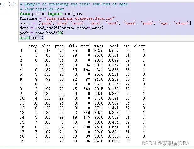
There is no substitute for looking at the raw data. Looking at the raw data can reveal insights that you cannot get any other way. It can also plant seeds that may later grow into ideas on how to better pre-process and handle the data for machine learning tasks. You can review the first 20 rows of your data using the head() function on the Pandas DataFrame.
# Example of reviewing the first few rows of data
# View first 20 rows
from pandas import read_csv
filename = "pima-indians-diabetes.data.csv"
names = ['preg','plas','pres', 'skin', 'test', 'mass', 'pedi', 'age', 'class']
data = read_csv(filename, names=names)
peek = data.head(20)
print(peek)
You can see that the first column lists the row number, which is handy for referencing a specific observation.
1.2 Dimensions of Your Data
You must have a very good handle on how much data you have, both in terms of rows and columns.
- Too many rows and algorithms may take too long to train. Too few and perhaps you do not have enough data to train the algorithms
- Too many features and some algorithms can be distracted or suffer poor performance due to the curse of dimensionality.
You can review the shape and size of your dataset by printing the shape property on the Pandas DataFrame.
# Example of reviewing the shape of the data
# Dimension of your data
from pandas import read_csv
filename = "pima-indians-diabetes.data.csv"
names = ['preg','plas','pres','skin','test','mass','pedi','age','class']
data = read_csv(filename, names=names)
shape = data.shape
print(shape)
The results are listed in rows then columns. You can see that the dataset has 768 rows and 9 columns.
(768, 9)
1.3 Data Type For Each Attribute
The type of each attribute is important. Strings may need to be converted to floating point values or integers to represent categorical or ordinal values. You can get an idea of the types of attributes by peeking at the raw data, as above. You can also list the data types used by the DataFrame to characterize each attribute using the dtypes property.
# Data Types for Each Attribute
from pandas import read_csv
filename = "pima-indians-diabetes.data.csv"
names = ['preg','plas','pres','skin','test','mass','pedi','age','class']
data = read_csv(filename, names=names)
types = data.dtypes
print(types)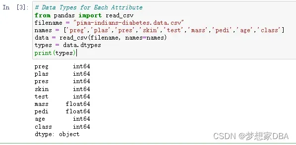
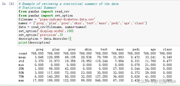
1.4 Descriptive Statistics
Descriptive statistics can give you great insight into the shape of each attribute. Often you can create more summaries than you have time to review. The describe() function on the Pandas DataFrame lists 8 statistical properties of each attribute. They are:
- Count
- Mean
- Standard Deviation
- Minimum Value
- 25th Percentile
- 50th Percentile(Median)
- 75th Percentile
- Maximum Value
# Example of reviewing a statistical summary of the data
# Statistical Summary
from pandas import read_csv
from pandas import set_option
filename = "pima-indians-diabetes.data.csv"
names = ['preg','plas','pres','skin','test','mass','pedi','age','class']
data = read_csv(filename, names=names)
set_option('display.width',100)
set_option('precision',3)
description = data.describe()
print(description)
You can see that you do get a lot of data. You will note some calls to pandas.set_option() in the recipe to change the precision of the numbers and the preferred width of the output. This is to make it more readable for this example. When describing your data this way, it is worth taking some time and reviewing observations from the results. This might include the presence of NA values for missing data or surprising distributions for attributes.
1.5 Class Distribution(Classification Only)
On classification problems you need to know how balanced the class values are. Highly imbalanced problems (a lot more observations for one class than another) are common and may need special handling in the data preparation stage of your project. You can quickly get an idea of the distribution of the class attribute in Pandas.
# Class Distribution
from pandas import read_csv
filename = "pima-indians-diabetes.data.csv"
names = ['preg','plas','pres','skin','test','mass','pedi','age','class']
data = read_csv(filename, names=names)
class_counts = data.groupby('class').size()
print(class_counts)
You can see that there are nearly double the number of observations with class 0 (no onset of diabetes) than there are with class 1 (onset of diabetes).
class
0    500
1    268
dtype: int64
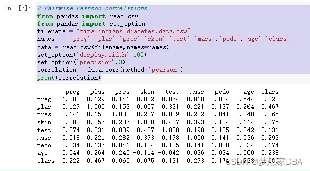
1.6 Correlations Between Attributes
Correlation refers to the relationship between two variables and how they may or may not change together. The most common method for calculating correlation is Pearson’s Correlation Coefficient, that assumes a normal distribution of the attributes involved. A correlation of -1 or 1 shows a full negative or positive correlation respectively. Whereas a value of 0 shows no correlation at all. Some machine learning algorithms like linear and logistic regression can suffer poor performance if there are highly correlated attributes in your dataset. As such, it is a good idea to review all of the pairwise correlations of the attributes in your dataset. You can use the corr() function on the Pandas DataFrame to calculate a correlation matrix.
# Pairwise Pearson correlations
from pandas import read_csv
from pandas import set_option
filename = "pima-indians-diabetes.data.csv"
names = ['preg','plas','pres','skin','test','mass','pedo','age','class']
data = read_csv(filename,names=names)
set_option('display.width',100)
set_option('precision',3)
correlation = data.corr(method='pearson')
print(correlation)
The matrix lists all attributes across the top and down the side, to give correlation between all pairs of attributes (twice, because the matrix is symmetrical). You can see the diagonal line through the matrix from the top left to bottom right corners of the matrix shows perfect correlation of each attribute with itself.
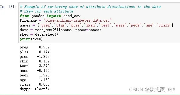
1.7 Skew of Univariate Distributions
Skew refers to a distribution that is assumed Gaussian (normal or bell curve) that is shifted or squashed in one direction or another. Many machine learning algorithms assume a Gaussian distribution. Knowing that an attribute has a skew may allow you to perform data preparation to correct the skew and later improve the accuracy of your models. You can calculate the skew of each attribute using the skew() function on the Pandas DataFrame.
# Example of reviewing skew of attribute distributions in the data
# Skew for each attribute
from pandas import read_csv
filename = "pima-indians-diabetes.data.csv"
names = ['preg','plas','pres','skin','test','mass','pedi','age','class']
data = read_csv(filename, names=names)
skew = data.skew()
print(skew)
The skew result show a positive (right) or negative (left) skew. Values closer to zero show less skew.
1.8 Tips To Remember
This section gives you some tips to remeber when reviewing your data using summary stastistics.
- Review the numbers . Generating the summary statistics is not enough. Take a moment to pause, read and really think about the numbers you are seeing.
- Ask why. Review your numbers and ask a lot of questions.How and why are you seeing specific numbers.Think about how the numbers relate to the problem domain in general and specific entities that observations relate to .
- Write down ideas. Write down your observations and ideas.Keep a small text file or note pad and jot down all of the ideas for how variables may relate, for what numbers mean, and ideas for techniques to try later.The things you write down now while the data is fresh will be very valuable later when you are trying to think up new things to try.
1.9 Summary
In this chapter you discovered the importance of describing your dataset before you start work on your machine learning project. You discovered 7 different ways to summarize your dataset using Python and Pandas:
- Peek At Your Data.
- Dimensions of Your Data.
- Data Types.
- Class Distribution.
- Data Summary.
- Correlations.
- Skewness.
文章出处登录后可见!