Pytorch 神经网络实践(随后复制到上一篇blog)

1. 定义神经网络结构 (2种方法)

import torch
import torch.nn as nn
import torch.nn.functional as F
from torchsummary import summary

# 定义网络类
class Net1(nn.Module):
    def __init__ (self):
        super(Net1, self).__init__()
        #定义第一层卷积层, 输入维度=1, 输出维度=6, kernel_size=3 卷积核大小3*3
        self.conv1 = nn.Conv2d(1, 6, 3)
        #定义第二层卷积层, 输入维度=6, 输出维度=16, 卷积核大小3*3
        self.conv2 = nn.Conv2d(6, 16, 3)
        #定义第三层全连接神经网络
        self.fc1 = nn.Linear(16*6*6, 120) #576=16*6*6？？
        self.fc2 = nn.Linear(120, 84)
        self.fc3 = nn.Linear(84, 10) #输出是10分类
    def forward(self, x):
        #注意:任意卷积层后面要加激活层, 池化层
        x = F.max_pool2d(F.relu(self.conv1(x)), (2, 2)) #(2, 2)??
        x = F.max_pool2d(F.relu(self.conv2(x)), 2)
        #经过卷积层的处理后，张量要进入全连接层，进入前需要调整张量的形状
        x = x.view(-1, self.num_flat_features(x))
        x = F.relu(self.fc1(x))
        x = F.relu(self.fc2(x))
        x = self.fc3(x)
        return x

    def num_flat_features(self, x):
        size = x.size()[1:]
        num_features = 1
        for s in size:
            num_features *= s
        return num_features

# Method 1_Net
net1 = Net1()
print(net1)

# Method 2_Net
#定义网络结构
net2 = nn.Sequential(
            nn.Conv2d(1, 6, kernel_size=3),
            nn.MaxPool2d(2, stride=2),
            nn.ReLU(True),
            nn.Conv2d(6, 16, kernel_size=3),
            nn.MaxPool2d(2, stride=2),
            nn.ReLU(True))
summary(net2, (1, 512, 512), batch_size=1, device="cpu")

运行结果：

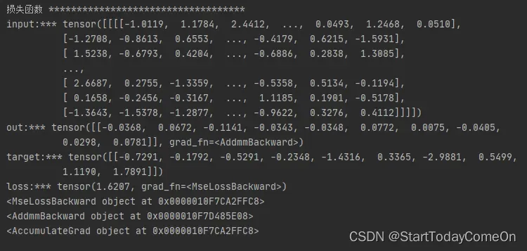
2. 损失函数

# input size 4D tensor = [nSample, nChannels, Height, Width]; 3D转4D tensor input.unsqueeze(0)
input = torch.randn(1, 1, 32, 32)
out = net1(input)
# output size [10 class], so target size [10 class]
target = torch.randn(10)
target = target.view(1, -1)
criterion = nn.MSELoss()
loss = criterion(out, target)
print('input:***', input)
print('out:***', out)
print('target:***', target)
print('loss:***', loss)
# 反向传播
# 关于方向传播的链条: 如果我们跟踪loss反向传播的方向，使用arad fn属性打印，将可以看到一张完整的计算图如下:
# input -> conv2d -> relu-> maxpoo12d-> conv2d-> relu-> maxpool2d-> view -> linear -> relu-> linear-> relu-> linear -> MSELOSS -> loss
# 当调用lossbackward()时，整张计算图将对loss进行自动求导，所有属性requires_grad=True的Tensors都将参与梯度求导的运算,并将梯度累加到Tensors中的grad属性中.
print(loss.grad_fn) # MSELOSS
print(loss.grad_fn.next_functions[0][0]) #Linear
print(loss.grad_fn.next_functions[0][0].next_functions[0][0]) #ReLU

运行结果：

参考视频课程：   P16-2.1Pytorch构建神经网络-第2步-损失函数_哔哩哔哩_bilibili