- 🍨 本文为🔗365天深度学习训练营 中的学习记录博客
- 🍦 参考文章地址: 365天深度学习训练营-第7周:咖啡豆识别
- 🍖 作者:K同学啊
一、前期工作
1.设置GPU
import tensorflow as tf

gpus = tf.config.list_physical_devices("GPU")

if gpus:
    tf.config.experimental.set_memory_growth(gpus[0], True)  #设置GPU显存用量按需使用
    tf.config.set_visible_devices([gpus[0]],"GPU")
2. 导入数据
from tensorflow       import keras
from tensorflow.keras import layers,models
import numpy             as np
import matplotlib.pyplot as plt
import os,PIL,pathlib

data_dir = "./49-data/"
data_dir = pathlib.Path(data_dir)
image_count = len(list(data_dir.glob('*/*.png')))
print("图片总数为:",image_count)图片总数为: 1200二、数据预处理
1. 加载数据
batch_size = 32
img_height = 224
img_width = 224
train_ds = tf.keras.preprocessing.image_dataset_from_directory(
data_dir,
validation_split=0.2,
subset="training",
seed=123,
image_size=(img_height, img_width),
batch_size=batch_size)Found 1200 files belonging to 4 classes.
Using 960 files for training.
val_ds = tf.keras.preprocessing.image_dataset_from_directory(
    data_dir,
    validation_split=0.2,
    subset="validation",
    seed=123,
    image_size=(img_height, img_width),
    batch_size=batch_size)
Found 1200 files belonging to 4 classes.
Using 240 files for validation.class_names = train_ds.class_names
print(class_names)['Dark', 'Green', 'Light', 'Medium']2. 可视化数据
plt.figure(figsize=(10, 4))  # 图形的宽为10高为5

for images, labels in train_ds.take(1):
    for i in range(10):

        ax = plt.subplot(2, 5, i + 1)

        plt.imshow(images[i].numpy().astype("uint8"))
        plt.title(class_names[labels[i]])

        plt.axis("off")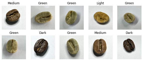
for image_batch, labels_batch in train_ds:
    print(image_batch.shape)
    print(labels_batch.shape)
    break
(32, 224, 224, 3)
(32,)3. 配置数据集
AUTOTUNE = tf.data.AUTOTUNE

train_ds = train_ds.cache().shuffle(1000).prefetch(buffer_size=AUTOTUNE)
val_ds   = val_ds.cache().prefetch(buffer_size=AUTOTUNE)
normalization_layer = layers.experimental.preprocessing.Rescaling(1./255)
train_ds = train_ds.map(lambda x, y: (normalization_layer(x), y))
val_ds = val_ds.map(lambda x, y: (normalization_layer(x), y))image_batch, labels_batch = next(iter(val_ds))
first_image = image_batch[0]
# 查看归一化后的数据
print(np.min(first_image), np.max(first_image))0.0 1.0
三、构建VGG-16网络
VGG优缺点分析:
- VGG优点
VGG的结构非常简洁,整个网络都使用了同样大小的卷积核尺寸(3×3)和最大池化尺寸(2×2)。
- VGG缺点
1)训练时间过长,调参难度大。2)需要的存储容量大,不利于部署。例如存储VGG-16权重值文件的大小为500多MB,不利于安装到嵌入式系统中。
1. 官方模型
# model = tf.keras.applications.VGG16(weights='imagenet')
# model.summary()
2. 自建模型
from tensorflow.keras import layers, models, Input
from tensorflow.keras.models import Model
from tensorflow.keras.layers import Conv2D, MaxPooling2D, Dense, Flatten, Dropout

def VGG16(nb_classes, input_shape):
    input_tensor = Input(shape=input_shape)
    # 1st block
    x = Conv2D(64, (3,3), activation='relu', padding='same',name='block1_conv1')(input_tensor)
    x = Conv2D(64, (3,3), activation='relu', padding='same',name='block1_conv2')(x)
    x = MaxPooling2D((2,2), strides=(2,2), name = 'block1_pool')(x)
    # 2nd block
    x = Conv2D(128, (3,3), activation='relu', padding='same',name='block2_conv1')(x)
    x = Conv2D(128, (3,3), activation='relu', padding='same',name='block2_conv2')(x)
    x = MaxPooling2D((2,2), strides=(2,2), name = 'block2_pool')(x)
    # 3rd block
    x = Conv2D(256, (3,3), activation='relu', padding='same',name='block3_conv1')(x)
    x = Conv2D(256, (3,3), activation='relu', padding='same',name='block3_conv2')(x)
    x = Conv2D(256, (3,3), activation='relu', padding='same',name='block3_conv3')(x)
    x = MaxPooling2D((2,2), strides=(2,2), name = 'block3_pool')(x)
    # 4th block
    x = Conv2D(512, (3,3), activation='relu', padding='same',name='block4_conv1')(x)
    x = Conv2D(512, (3,3), activation='relu', padding='same',name='block4_conv2')(x)
    x = Conv2D(512, (3,3), activation='relu', padding='same',name='block4_conv3')(x)
    x = MaxPooling2D((2,2), strides=(2,2), name = 'block4_pool')(x)
    # 5th block
    x = Conv2D(512, (3,3), activation='relu', padding='same',name='block5_conv1')(x)
    x = Conv2D(512, (3,3), activation='relu', padding='same',name='block5_conv2')(x)
    x = Conv2D(512, (3,3), activation='relu', padding='same',name='block5_conv3')(x)
    x = MaxPooling2D((2,2), strides=(2,2), name = 'block5_pool')(x)
    # full connection
    x = Flatten()(x)
    x = Dense(4096, activation='relu',  name='fc1')(x)
    x = Dense(4096, activation='relu', name='fc2')(x)
    output_tensor = Dense(nb_classes, activation='softmax', name='predictions')(x)

    model = Model(input_tensor, output_tensor)
    return model

model=VGG16(len(class_names), (img_width, img_height, 3))
model.summary()
Model: "model" _________________________________________________________________ Layer (type) Output Shape Param # ================================================================= input_1 (InputLayer) [(None, 224, 224, 3)] 0 _________________________________________________________________ block1_conv1 (Conv2D) (None, 224, 224, 64) 1792 _________________________________________________________________ block1_conv2 (Conv2D) (None, 224, 224, 64) 36928 _________________________________________________________________ block1_pool (MaxPooling2D) (None, 112, 112, 64) 0 _________________________________________________________________ block2_conv1 (Conv2D) (None, 112, 112, 128) 73856 _________________________________________________________________ block2_conv2 (Conv2D) (None, 112, 112, 128) 147584 _________________________________________________________________ block2_pool (MaxPooling2D) (None, 56, 56, 128) 0 _________________________________________________________________ block3_conv1 (Conv2D) (None, 56, 56, 256) 295168 _________________________________________________________________ block3_conv2 (Conv2D) (None, 56, 56, 256) 590080 _________________________________________________________________ block3_conv3 (Conv2D) (None, 56, 56, 256) 590080 _________________________________________________________________ block3_pool (MaxPooling2D) (None, 28, 28, 256) 0 _________________________________________________________________ block4_conv1 (Conv2D) (None, 28, 28, 512) 1180160 _________________________________________________________________ block4_conv2 (Conv2D) (None, 28, 28, 512) 2359808 _________________________________________________________________ block4_conv3 (Conv2D) (None, 28, 28, 512) 2359808 _________________________________________________________________ block4_pool (MaxPooling2D) (None, 14, 14, 512) 0 _________________________________________________________________ block5_conv1 (Conv2D) (None, 14, 14, 512) 2359808 _________________________________________________________________ block5_conv2 (Conv2D) (None, 14, 14, 512) 2359808 _________________________________________________________________ block5_conv3 (Conv2D) (None, 14, 14, 512) 2359808 _________________________________________________________________ block5_pool (MaxPooling2D) (None, 7, 7, 512) 0 _________________________________________________________________ flatten (Flatten) (None, 25088) 0 _________________________________________________________________ fc1 (Dense) (None, 4096) 102764544 _________________________________________________________________ fc2 (Dense) (None, 4096) 16781312 _________________________________________________________________ predictions (Dense) (None, 4) 16388 ================================================================= Total params: 134,276,932 Trainable params: 134,276,932 Non-trainable params: 0 _________________________________________________________________
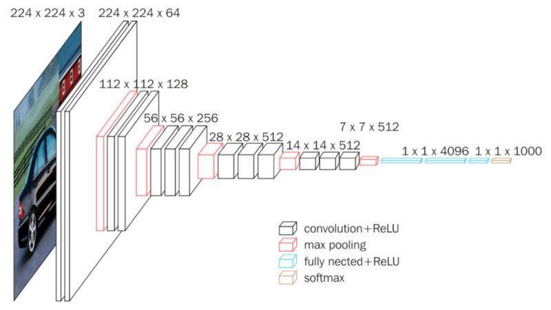
3. 网络结构图
结构说明:
- 13个卷积层(Convolutional Layer),分别用blockX_convX表示
- 3个全连接层(Fully connected Layer),分别用fcX与predictions表示
- 5个池化层(Pool layer),分别用blockX_pool表示
VGG-16包含了16个隐藏层(13个卷积层和3个全连接层),故称为VGG-16。
四、编译
# 设置初始学习率
initial_learning_rate = 1e-4

lr_schedule = tf.keras.optimizers.schedules.ExponentialDecay(
        initial_learning_rate,
        decay_steps=30,      # 敲黑板!!!这里是指 steps,不是指epochs
        decay_rate=0.92,     # lr经过一次衰减就会变成 decay_rate*lr
        staircase=True)

# 设置优化器
opt = tf.keras.optimizers.Adam(learning_rate=initial_learning_rate)

model.compile(optimizer=opt,
              loss=tf.keras.losses.SparseCategoricalCrossentropy(from_logits=True),
              metrics=['accuracy'])
五、训练模型
epochs = 20

history = model.fit(
    train_ds,
    validation_data=val_ds,
    epochs=epochs
)
30/30 [==============================] - 7s 236ms/step - loss: 0.1117 - accuracy: 0.9638 - val_loss: 0.0425 - val_accuracy: 0.9875
六、可视化结果
acc = history.history['accuracy']
val_acc = history.history['val_accuracy']

loss = history.history['loss']
val_loss = history.history['val_loss']

epochs_range = range(epochs)

plt.figure(figsize=(12, 4))
plt.subplot(1, 2, 1)
plt.plot(epochs_range, acc, label='Training Accuracy')
plt.plot(epochs_range, val_acc, label='Validation Accuracy')
plt.legend(loc='lower right')
plt.title('Training and Validation Accuracy')

plt.subplot(1, 2, 2)
plt.plot(epochs_range, loss, label='Training Loss')
plt.plot(epochs_range, val_loss, label='Validation Loss')
plt.legend(loc='upper right')
plt.title('Training and Validation Loss')
plt.show()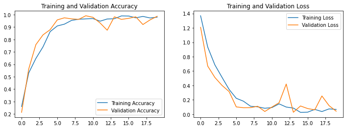
from PIL import Image
import numpy as np

img = np.array(Image.open("./49-data/Green/green (102).png"))  #这里选择你需要预测的图片
image = tf.image.resize(img, [img_height, img_width])

img_array = tf.expand_dims(image, 0)

predictions = model.predict(img_array) # 这里选用你已经训练好的模型
print("预测结果为:",class_names[np.argmax(predictions)])
预测结果为: Green文章出处登录后可见!
已经登录?立即刷新