今天接着单细胞文章的内容:
前面几期主要说了下每个阶段出现图的个性化修饰,后面依然如此,有需要值得单拎出来说的,我们也是会讲到。
细胞分群命名完成之后,大多数研究会关注各个样本细胞群的比例,尤其是免疫学的研究中,各群免疫细胞比例的变化是比较受关注的。所以这里说说细胞群比例的计算,以及如何可视化。
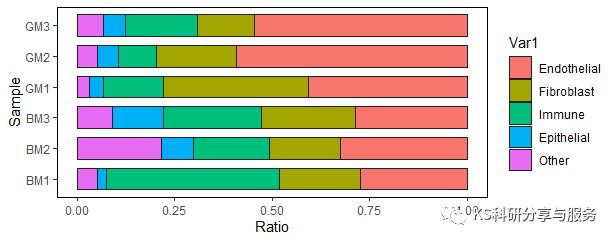
1、堆叠柱状图
这是比较普通也是最常用的细胞比例可视化方法。这种图在做微生物菌群的研究中非常常见。具体的思路是计算各个样本中细胞群的比例,形成数据框之后转化为长数据,用ggplot绘制即可。
table(scedata$orig.ident)#查看各组细胞数
#BM1  BM2  BM3  GM1  GM2  GM3
#2754  747 2158 1754 1528 1983
prop.table(table(Idents(scedata)))
table(Idents(scedata), scedata$orig.ident)#各组不同细胞群细胞数
#BM1  BM2  BM3  GM1  GM2  GM3
#  Endothelial  752  244  619  716  906 1084
#  Fibroblast   571  135  520  651  312  286
#  Immune      1220  145  539  270  149  365
#  Epithelial    69   62  286   62   82  113
#  Other        142  161  194   55   79  135
Cellratio <- prop.table(table(Idents(scedata), scedata$orig.ident), margin = 2)#计算各组样本不同细胞群比例
Cellratio
#BM1        BM2        BM3        GM1        GM2        GM3
#  Endothelial 0.27305737 0.32663989 0.28683967 0.40820981 0.59293194 0.54664650
#  Fibroblast  0.20733479 0.18072289 0.24096386 0.37115165 0.20418848 0.14422592
#  Immune      0.44299201 0.19410977 0.24976830 0.15393387 0.09751309 0.18406455
#  Epithelial  0.02505447 0.08299866 0.13253012 0.03534778 0.05366492 0.05698437
#  Other       0.05156137 0.21552878 0.08989805 0.03135690 0.05170157 0.06807867
Cellratio <- as.data.frame(Cellratio)
colourCount = length(unique(Cellratio$Var1))
library(ggplot2)
ggplot(Cellratio) +
  geom_bar(aes(x =Var2, y= Freq, fill = Var1),stat = "identity",width = 0.7,size = 0.5,colour = '#222222')+
  theme_classic() +
  labs(x='Sample',y = 'Ratio')+
  coord_flip()+
  theme(panel.border = element_rect(fill=NA,color="black", size=0.5, linetype="solid"))
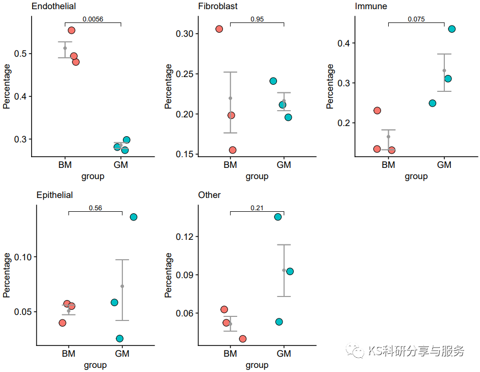
2、批量统计图
很多时候,我们不仅想关注各个样本中不同细胞群的比例,而且更想指导他们在不同样本之中的变化是否具有显著性。这时候,除了要计算细胞比例外,还需要进行显著性检验。这里我们提供了一种循环的做法,可以批量完成不同样本细胞比例的统计分析及可视化。
table(scedata$orig.ident)#查看各组细胞数
prop.table(table(Idents(scedata)))
table(Idents(scedata), scedata$orig.ident)#各组不同细胞群细胞数
Cellratio <- prop.table(table(Idents(scedata), scedata$orig.ident), margin = 2)#计算各组样本不同细胞群比例
Cellratio <- data.frame(Cellratio)
library(reshape2)
cellper <- dcast(Cellratio,Var2~Var1, value.var = "Freq")#长数据转为宽数据
rownames(cellper) <- cellper[,1]
cellper <- cellper[,-1]


###添加分组信息
sample <- c("BM1","BM2","BM3","GM1","GM2","GM3")
group <- c("BM","BM","BM","GM","GM","GM")
samples <- data.frame(sample, group)#创建数据框

rownames(samples)=samples$sample
cellper$sample <- samples[rownames(cellper),'sample']#R添加列
cellper$group <- samples[rownames(cellper),'group']#R添加列

###作图展示
pplist = list()
sce_groups = c('Endothelial','Fibroblast','Immune','Epithelial','Other')
library(ggplot2)
library(dplyr)
library(ggpubr)
for(group_ in sce_groups){
  cellper_  = cellper %>% select(one_of(c('sample','group',group_)))#选择一组数据
  colnames(cellper_) = c('sample','group','percent')#对选择数据列命名
  cellper_$percent = as.numeric(cellper_$percent)#数值型数据
  cellper_ <- cellper_ %>% group_by(group) %>% mutate(upper =  quantile(percent, 0.75),
                                                      lower = quantile(percent, 0.25),
                                                      mean = mean(percent),
                                                      median = median(percent))#上下分位数
  print(group_)
  print(cellper_$median)

  pp1 = ggplot(cellper_,aes(x=group,y=percent)) + #ggplot作图
    geom_jitter(shape = 21,aes(fill=group),width = 0.25) +
    stat_summary(fun=mean, geom="point", color="grey60") +
    theme_cowplot() +
    theme(axis.text = element_text(size = 10),axis.title = element_text(size = 10),legend.text = element_text(size = 10),
          legend.title = element_text(size = 10),plot.title = element_text(size = 10,face = 'plain'),legend.position = 'none') +
    labs(title = group_,y='Percentage') +
    geom_errorbar(aes(ymin = lower, ymax = upper),col = "grey60",width =  1)

  ###组间t检验分析
  labely = max(cellper_$percent)
  compare_means(percent ~ group,  data = cellper_)
  my_comparisons <- list( c("GM", "BM") )
  pp1 = pp1 + stat_compare_means(comparisons = my_comparisons,size = 3,method = "t.test")
  pplist[[group_]] = pp1
}

library(cowplot)
plot_grid(pplist[['Endothelial']],
          pplist[['Fibroblast']],
          pplist[['Immune']],
          pplist[['Epithelial']],
          pplist[['Other']])
好了,以上就是我们的分享了,起到抛砖引玉的效果,还有很多其他的展示方法,不必全都会,中意就好。
更多内容请至我的个人公众号《KS科研分享与服务》
文章出处登录后可见!
已经登录?立即刷新