Vision Transformer (ViT)初识:原理详解及代码
参考资源
论文:An Image is Worth 16×16 Words: Transformers for Image Recognition at Scale
代码:https://github.com/google-research/vision_transformer(原论文对应源码)
代码:https://github.com/lucidrains/vit-pytorch
知乎:Vision Transformer
知乎:ViT(Vision Transformer)解析
CSDN:Vision Transformer详解
前言
Transformer最初提出是针对NLP领域的。
Vision Transformer将CV和NLP领域知识结合起来,对原始图片进行分块,展平成序列,输入进原始Transformer模型的编码器Encoder部分,最后接入一个全连接层对图片进行分类。
1. 整体架构
原论文中 Vision Transformer(ViT) 的模型框架。由三个模块组成:
- Linear Projection of Flattened Patches(Embedding层)
- Transformer Encoder(图右侧更加详细结构)
- MLP Head(最终用于分类的层)
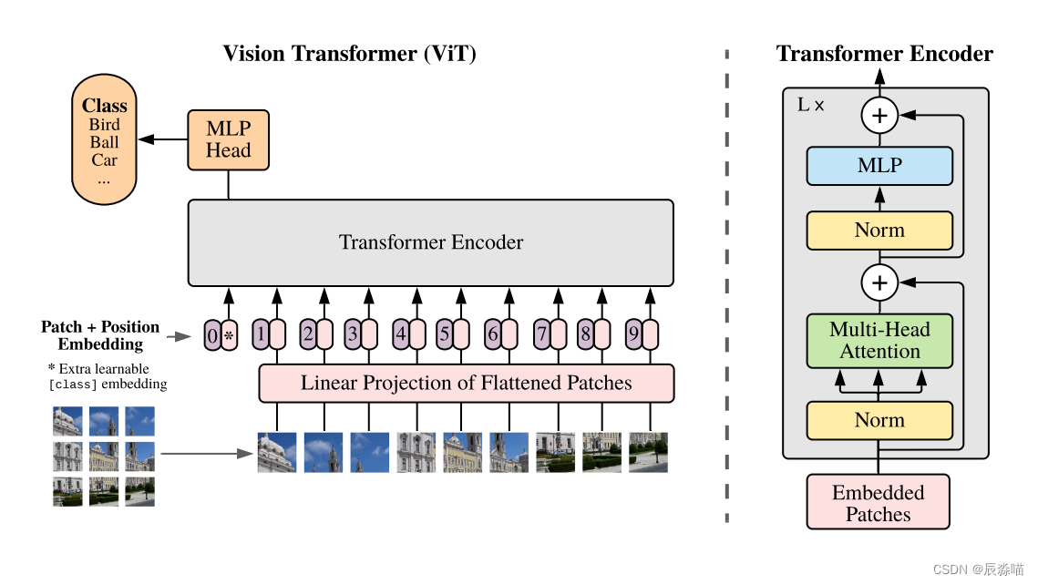
1.1 Embedding层
Transformer模块的输入:token(向量)序列,即二维矩阵[num_token, token_dim]
对于图像数据:将 [H, W, C] 三维矩阵通过一个Embedding层进行变换。
先对图片作分块,再进行展平
首先将一张图片按给定大小分成一堆Patches,分块的数目为:
对每个图片块展平成一维向量,每个向量大小为
以ViT-B/16为例:
将输入图片(224×224)按照16×16大小的Patch进行划分,会得到196个Patches.
接着通过线性映射将每个Patch映射到一维向量中,每个Patche数据shape为 [16, 16, 3] 通过映射得到一个长度为 768 的向量(后面都直接称为 token)。
在代码实现中,通过一个卷积层来实现。 以ViT-B/16为例,使用一个卷积核大小为16×16,步距为16,卷积核个数为768的卷积来实现。通过卷积[224, 224, 3] -> [14, 14, 768],然后把H以及W两个维度展平即可[14, 14, 768] -> [196, 768],此时正好变成了一个二维矩阵,正是Transformer想要的。
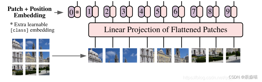
在输入Transformer Encoder之前注意需要加上 [class]token 以及Position Embedding。 其中:
class token
假设我们按照论文切成了9块,但是在输入的时候变成了10个向量。这是人为增加的一个向量。
因为传统的Transformer采取的是类似seq2seq编解码的结构 而ViT只用到了Encoder编码器结构,缺少了解码的过程,假设你9个向量经过编码器之后,你该选择哪一个向量进入到最后的分类头呢?因此这里作者给了额外的一个用于分类的向量,与输入进行拼接。
[class]token是一个可训练的参数,数据格式和其他token一样都是一个向量
以ViT-B/16为例,就是: 一个长度为768的向量,与之前从图片中生成的tokens拼接在一起,
Cat([1, 768], [196, 768]) -> [197, 768]
Position Embedding
Position Embedding采用的是一个可训练的参数(1D Pos. Emb.),是直接叠加在tokens上的(add),所以shape要一样。
以ViT-B/16为例,刚刚拼接[class]token后shape是[197, 768],那么这里的Position Embedding的shape也是[197, 768]。
1.2 Transformer Encoder层
重复堆叠 Encoder Block L次,Encoder Block组成:
- Layer Norm
主要是针对NLP领域提出的,是对每个token进行Norm处理 - Multi-Head Attention
多头注意力,可以参考上篇 - Dropout/DropPath
在原论文的代码中是直接使用的Dropout层,在但rwightman实现的代码中使用的是DropPath(stochastic depth),可能后者会更好一点。 - MLP Block
全连接+GELU激活函数+Dropout
需要注意的是第一个全连接层会把输入节点个数翻4倍[197, 768] -> [197, 3072],第二个全连接层会还原回原节点个数[197, 3072] -> [197, 768]

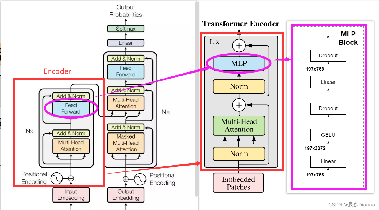
MLP block ,MLP head 和 FFN
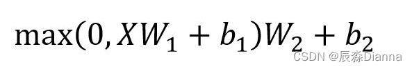
Feed Forward
Feed Forward 层是一个两层的全连接层,第一层的激活函数为 Gelu,第二层不使用激活函数,对应的公式如下。
Transformer 结构里的 Feed Forward 实际上就是 ViT (VisionTransformer) 结构里的 MLP Block,下图用粉色圈标出,具体结构为右侧粉色框,是一个全连接网络,包含两个线性变换和一个非线性函数
左边Transformer 结构里的 Encoder 用红色框标出,对应右边红色框的 ViT (VisionTransformer),因为ViT不包含Decorder
FeedForward 即 ViT 的 MLP Block 代码:
两个全连接中间夹个激活函数,可以是RELU或者GELU,加入了dropout
class FeedForward(nn.Module):
    def __init__(self, dim, hidden_dim, dropout = 0.):
        super().__init__()
        self.net = nn.Sequential(
            nn.Linear(dim, hidden_dim),
            nn.GELU(),
            nn.Dropout(dropout),
            nn.Linear(hidden_dim, dim),
            nn.Dropout(dropout)
        )
    def forward(self, x):
        return self.net(x)
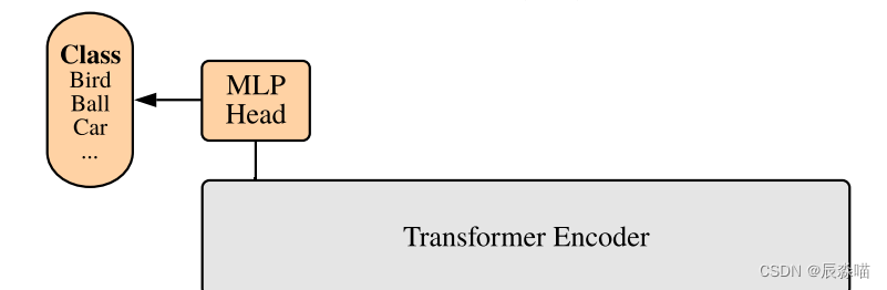
1.3 MLP head 分类层
MLP Head 是ViT 里用于分类的预测头,结构和代码如下,也是由LN 和线性层组成
MLP head 代码:
        self.mlp_head = nn.Sequential(
            nn.LayerNorm(dim),
            nn.Linear(dim, num_classes)
代码中,取token的第一个,也就是用于分类的token,输入到分类头里,得到最后的分类结果
即[197, 768]中抽取出[class]token对应的[1, 768]。
2. 代码解析
VIT Vision Transformer | 先从PyTorch代码了解
VIT(vision transformer)模型介绍+pytorch代码炸裂解析
ViT源码阅读-PyTorch
ViT 调用
import torch
from vit_pytorch import SimpleViT

import torch
from vit_pytorch import ViT

v = ViT(
    image_size = 256,     # width and height
    patch_size = 32,      # Number of patches.
    num_classes = 1000,   # Number of classes to classify.
    dim = 1024,           # Last dimension of output tensor after linear transformation
    depth = 6,            # Number of Transformer blocks.
    heads = 16,           # Number of heads in Multi-head Attention layer.
    mlp_dim = 2048        # Dimension of the MLP (FeedForward) layer.
    dropout = 0.1,
    emb_dropout = 0.1
)

img = torch.randn(1, 3, 256, 256)   # [batch, channel, height, width]
preds2 = v(img)                              # (1, 1000)
Class PreNorm:线性化
class PreNorm(nn.Module):
    def __init__(self, dim, fn):
        super().__init__()
        self.norm = nn.LayerNorm(dim)
        self.fn = fn
    def forward(self, x, **kwargs):
        # 先LN
        return self.fn(self.norm(x), **kwargs)
Class FeedForward:即 MLP Block
# 两个全连接中间夹个激活函数,可以是RELU或者GELU,加入了dropout
class FeedForward(nn.Module):
    def __init__(self, dim, hidden_dim, dropout = 0.):
        super().__init__()
        self.net = nn.Sequential(
            nn.Linear(dim, hidden_dim),
            nn.GELU(),
            nn.Dropout(dropout),
            nn.Linear(hidden_dim, dim),
            nn.Dropout(dropout)
        )
    def forward(self, x):
        return self.net(x)
Class Attention:注意力模块
class Attention(nn.Module):
    def __init__(self, dim, heads = 8, dim_head = 64, dropout = 0.):
        super().__init__()
        inner_dim = dim_head *  heads
        project_out = not (heads == 1 and dim_head == dim)

        self.heads = heads
        self.scale = dim_head ** -0.5   # 论文里的\sqrt{d_k}

        self.attend = nn.Softmax(dim = -1)
        self.dropout = nn.Dropout(dropout)

        self.to_qkv = nn.Linear(dim, inner_dim * 3, bias = False)

        self.to_out = nn.Sequential(
            nn.Linear(inner_dim, dim),
            nn.Dropout(dropout)
        ) if project_out else nn.Identity()

    def forward(self, x):
        # 输入 x -> (batch, 197, 768)即(batch, num_patch + 1, hid_dims)
        # 按照最后一维(特征维度)分成3块,分别对应QKV
        # chunk后是一个tuple,即(q, k, v)
        qkv = self.to_qkv(x).chunk(3, dim = -1)
        # q, k, v都做维度变换,(batch, 197, 768) -> (batch, 12, 197, 768 / 12 = 64)
        # 12是head的数量,目的是做**多头**注意力机制
        q, k, v = map(lambda t: rearrange(t, 'b n (h d) -> b h n d', h = self.heads), qkv)
        # Q @ K^T  /  \sqrt{d_k}
        dots = torch.matmul(q, k.transpose(-1, -2)) * self.scale

        attn = self.attend(dots)
        attn = self.dropout(attn)

        out = torch.matmul(attn, v)
        # 把多头拼回去 -> (batch, 197, 768)
        out = rearrange(out, 'b h n d -> b n (h d)')
        return self.to_out(out)
Class Transformer :Encoder
class Transformer(nn.Module):
    def __init__(self, dim, depth, heads, dim_head, mlp_dim, dropout = 0.):
        super().__init__()
        self.layers = nn.ModuleList([])
        for _ in range(depth):
            self.layers.append(nn.ModuleList([
                # 先对输入做lN,然后放到attention,然后和做lN之前的输入相加做一个残差链接;
                PreNorm(dim, Attention(dim, heads = heads, dim_head = dim_head, dropout = dropout)),
                # x->LayerNormalization->FeedForward线性层(即MLP block)->y, 然后这个y和输入的x相加,做残差连接。
                PreNorm(dim, FeedForward(dim, mlp_dim, dropout = dropout))
            ]))
    def forward(self, x):
        for attn, ff in self.layers:  # attn为Multi-head Attention,ff就是FeedForward
            x = attn(x) + x           # 残差连接,图片中的边线
            x = ff(x) + x
        return x
整体框架
class ViT(nn.Module):
    def __init__(self, *, image_size, patch_size, num_classes, dim, depth, heads, mlp_dim, pool = 'cls', channels = 3, dim_head = 64, dropout = 0., emb_dropout = 0.):
        super().__init__()
        image_height, image_width = pair(image_size)
        patch_height, patch_width = pair(patch_size)   # 默认为16   行和列上一共有224 / 16 = 14个patch

        assert image_height % patch_height == 0 and image_width % patch_width == 0, 'Image dimensions must be divisible by the patch size.'

        # # num patches -> (224 / 16) = 14, 14 * 14 = 196
        num_patches = (image_height // patch_height) * (image_width // patch_width)   # 分块数目: N = H *W/(P*P)
        # # path dim -> 3 * 16 * 16 = 768,和Bert-base一致
        patch_dim = channels * patch_height * patch_width
        assert pool in {'cls', 'mean'}, 'pool type must be either cls (cls token) or mean (mean pooling)'

        # 步骤一:图像分块与映射。首先将图片分块,然后接一个线性层做映射
        #  [224, 224, 3] -> [14, 14, 768]  ——> # [14, 14, 768] -> [196, 768]
        self.to_patch_embedding = nn.Sequential(
            Rearrange('b c (h p1) (w p2) -> b (h w) (p1 p2 c)', p1 = patch_height, p2 = patch_width),
            nn.Linear(patch_dim, dim),
        )

        # pos_embedding:位置编码;cls_token:在序列最前面插入一个cls token作为分类输出
        # Cat([1, 768], [196, 768]) -> [197, 768]
        self.pos_embedding = nn.Parameter(torch.randn(1, num_patches + 1, dim))
        self.cls_token = nn.Parameter(torch.randn(1, 1, dim))
        self.dropout = nn.Dropout(emb_dropout)

        # 步骤二:Transformer Encoder结构来提特征 即  Transformer Encoder
        self.transformer = Transformer(dim, depth, heads, dim_head, mlp_dim, dropout)

        self.pool = pool
        self.to_latent = nn.Identity()

        # 线性层输出
        self.mlp_head = nn.Sequential(
            nn.LayerNorm(dim),
            nn.Linear(dim, num_classes)
        )

    def forward(self, img):
        x = self.to_patch_embedding(img)
        b, n, _ = x.shape

        # 1 x 1 x 768的CLS token重复至 batch x 1 x 768
        cls_tokens = repeat(self.cls_token, '1 1 d -> b 1 d', b = b)
        x = torch.cat((cls_tokens, x), dim=1)
        x += self.pos_embedding[:, :(n + 1)]   # 因为多了个CLS token所以要n+1
        x = self.dropout(x)
        # x.shape -> (batch, 196 + 1, 768)

        x = self.transformer(x)   # Transformer Encoder

        x = x.mean(dim = 1) if self.pool == 'mean' else x[:, 0]

        x = self.to_latent(x)
        return self.mlp_head(x)
本篇是Transformer 在视觉的应用 ViT 的原理和代码
ViT 的应用和变体的解析和代码参考下篇:
ViT 的应用和变体的解析和代码
Transformer 基本原理和知识参考上篇:
Transformer 初识:模型结构+attention原理详解
文章出处登录后可见!