目录

SQL

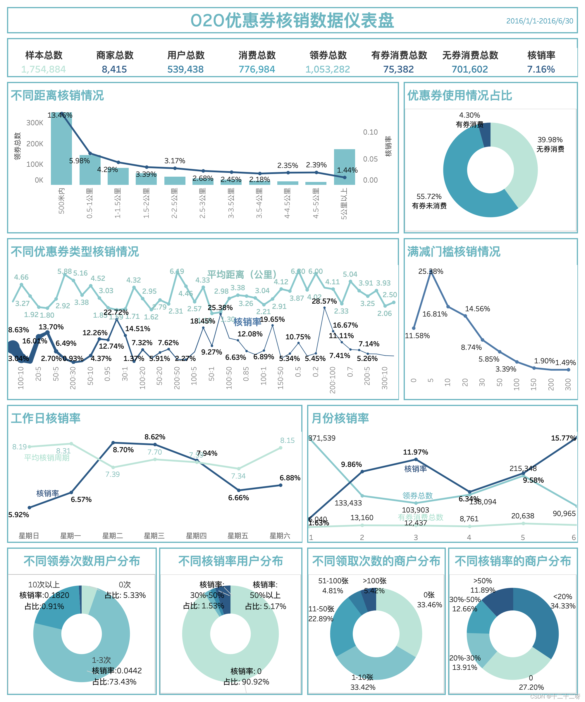
统计数据概况：计算样本总数、商家总数、用户总数、消费总数、领券总数等

select
    count(User_id) as '样本总数',
    count(distinct Merchant_id) as '商家总数',
    count(distinct User_id) as '用户总数',
    count(Date) as '消费总数',
    count(Date_received) as '领券总数',
    (select count(*) from ddm.offline_train as a where a.Date_received is not null and a.Date is not null) as '领券消费总数',
    (select count(*) from ddm.offline_train as a where a.Date_received is null and a.Date is not null) as '无券消费总数',
    (select count(*) from ddm.offline_train as a where a.Date_received is not null and a.Date is not null)/count(Date_received) as '核销率'
from ddm.offline_train

统计不同距离下：领券人数、用券消费人数、核销率

# 查找各距离的领券人数/用券消费人数/核销率
select
    Distance,
    count(Coupon_id) as get_coupons_num,
    sum(if(Date_received is not null and Date is not null,1,0)) as user_coupons_num,
    sum(if(Date_received is not null and Date is not null,1,0)) /count(Coupon_id) as use_coupons_rate
from ddm.offline_train
where Distance is not null
group by Distance
order by distance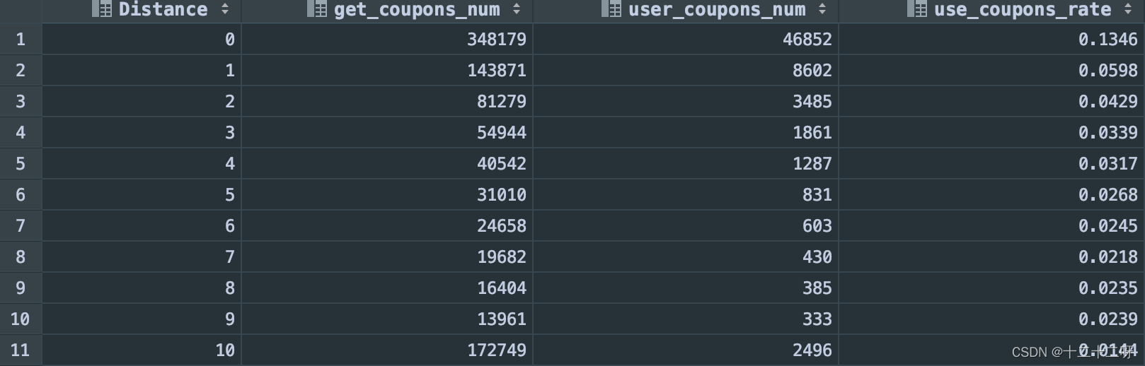

 消费券使用情况占比

# 消费券使用情况占比
with temp as (
    select
        case
            when Date_received is not null and Date is not null then '有券消费'
            when Date_received is not null and Date is null then '有券未消费'
            when Date_received is null and Date is not null then '无券消费'
        end as flag
    from ddm.offline_train
)
select
    flag as '优惠券使用情况',
    concat(round(count(flag)/(select count(*) from temp)*100,2),'%') as '百分比'
from temp
group by flag
order by count(flag)/(select count(*) from temp)

 with as 也叫做子查询部分，类似于一个视图或临时表，可以用来存储一部分的sql语句查询结果，必须和其他的查询语句一起使用，且中间不能有分号，目前在oracle、sql server、hive等均支持 with as 用法，但 mysql并不支持！

不同类型优惠券的核销情况和平均领取距离

# 不同优惠券类型的核销情况和平均领取距离
select
    Discount_rate as '折扣',
    avg(Distance) as '平均距离',
    count(Date_received) as '领券人数',
    sum(if(Date_received is not null and Date is not null,1,0)) as '有券消费人数',
    sum(if(Date_received is not null and Date is not null,1,0))/count(Date_received) as '核销率'
from ddm.offline_train
where Date_received is not null
group by Discount_rate
order by '有券消费人数' desc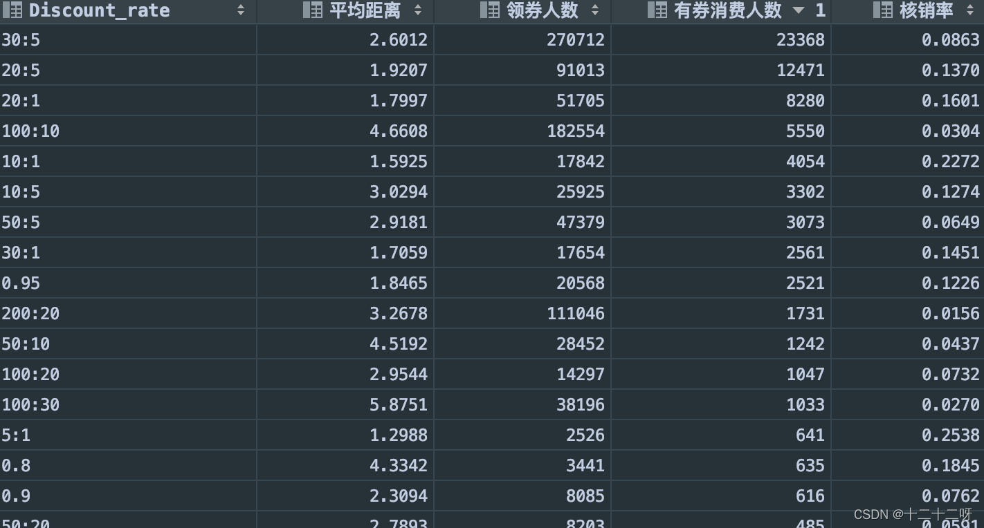

不同满减门槛的核销情况

# 不同满减门槛的核销情况
select
    mk as '门槛',
    count(*) as '领券数量',
    sum(if(Date is not null,1,0)) as '用券消费数量',
    concat(round(sum(if(Date is not null,1,0))/count(*)*100,2),'%') as '核销率'
from(select
         DATE,
         convert(if(Discount_rate like '%.%',0,Discount_rate),signed) as mk
    from ddm.offline_train) as aa
where mk is not null
group by mk
order by mk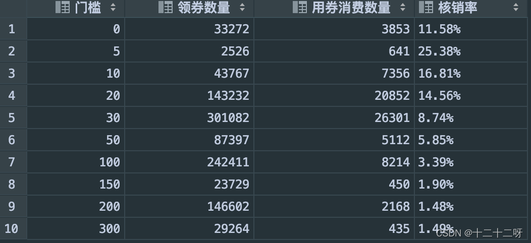

不同核销率的商家分布情况（占比）

# 不同核销率用户分布
with temp as (
    select
        Merchant_id,
        count(Date_received) as get_num,
        sum(if(Date is not null and Date_received is not null,1,0)) as use_num,
        sum(if(Date is not null and Date_received is not null,1,0))/count(Date_received) as Merchant_rate
    from ddm.offline_train
    where Date_received is not null
    group by Merchant_id
)
 
 
select
    tag,
    concat(round(count(*)/(select count(*) from temp)*100,2),'%') as Merchant_percent
from(
    select
        Merchant_id,
        case
            when Merchant_rate = 0 then '核销率：0'
            when Merchant_rate > 0 and Merchant_rate < 0.2 then '核销率：0-20%'
            when Merchant_rate >= 0.2 and Merchant_rate< 0.3 then '核销率：20%-30%'
            when Merchant_rate >= 0.3 and Merchant_rate< 0.5 then '核销率：30%-50%'
            when Merchant_rate >= 0.5 then '核销率：50%以上'
        end as tag
    from temp
    )aa
group by tag
order by Merchant_percent desc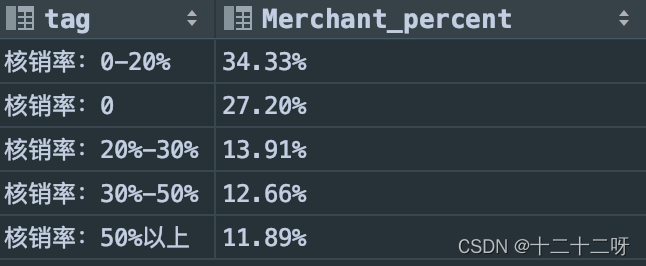

不同领券次数商家的分布情况（平均核销率/占比） 

# 不同领券次数用户分布-平均核销率/占比
with temp as (
    select
        Merchant_id,
        count(Date_received) as get_num,
        sum(if(Date is not null and Date_received is not null,1,0))/count(Date_received) as user_rate,
        sum(if(Date is not null and Date_received is not null,1,0)) as use_num,
        case
            when count(Date_received)>100 then '100次以上'
            when count(Date_received)=0 then '0次'
            when count(Date_received) between 1 and 10 then '1-10次'
            when count(Date_received) between 11 and 50 then '11-50次'
            when count(Date_received) between 51 and 100 then '51-100次'
            else '其他次'
        end as flag
    from ddm.offline_train
    group by Merchant_id
)
 
select
    flag as '被领券次数',
    concat(round(avg(user_rate)*100,2),'%') as Merchant_avg_use_rate,
    concat(round(count(*)/(select count(*) from temp)*100,2),'%') as Merchant_percent
from temp
group by flag
order by (count(*)/(select count(*) from temp)) desc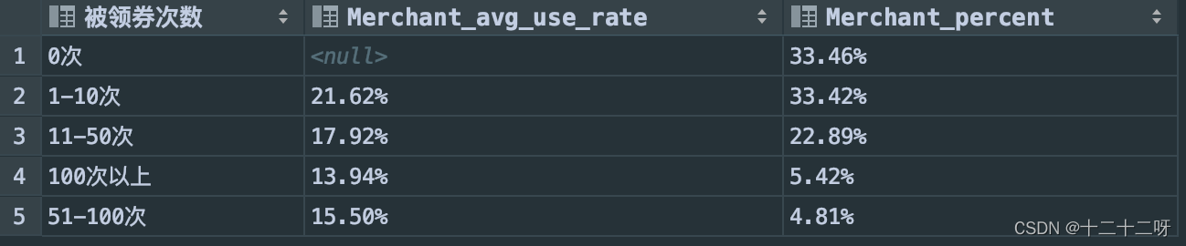

不同核销率用户分布（占比）

# 不同核销率用户分布
with temp as (
    select
        User_id,
        count(Date_received) as get_num,
        sum(if(Date is not null and Date_received is not null,1,0)) as use_num,
        sum(if(Date is not null and Date_received is not null,1,0))/count(Date_received) as user_rate
    from ddm.offline_train
    where Date_received is not null
    group by User_id
)
 
 
select
    tag,
    concat(round(count(*)/(select count(*) from temp)*100,2),'%') as user_percent
from(
    select
        User_id,
        case
            when user_rate = 0 then '核销率：0'
            when user_rate > 0 and user_rate < 0.3 then '核销率：0-30%'
            when user_rate >= 0.3 and user_rate< 0.5 then '核销率：30%-50%'
            when user_rate >= 0.5 then '核销率：50%以上'
        end as tag
    from temp
    )aa
group by tag
order by user_percent desc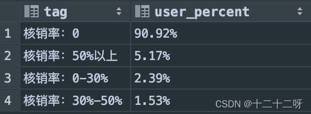

不同月份优惠券领券次数/核销次数/核销率

# 不同月份领券次数/核销次数/核销率
select
    `month`,
    coupons_get_num,
    coupons_use_num,
    concat(round(coupons_use_num/coupons_get_num*100,2),'%') as coupons_use_rate
from(select
        month(Date_received) as `month`,
        count(*) as coupons_get_num
    from ddm.offline_train
    where Date_received is not null
    group by month(Date_received)) as a
inner join(
    select
        month(Date) as `month`,
        count(*) as coupons_use_num
    from ddm.offline_train
    where Date_received is not null and Date is not null
    group by month(Date)
)as b using(`month`)
order by `month`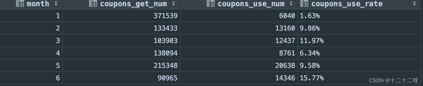

不同工作日的优惠券平均核销周期、核销率

# 工作日平均核销间隔、核销率
with get_coupons as(
    select
        weekday(Date_received)+1 as coupons_day,
        count(*) as coupons_get_num
    from ddm.offline_train
    where Date_received is not null
    group by weekday(Date_received)+1
),
use_coupons as(
    select
        weekday(Date)+1 as coupons_day,
        count(*) as coupons_use_num,
        round(avg(datediff(Date,Date_received)),2) as use_interval
    from ddm.offline_train
    where Date is not null and Date_received is not null
    group by weekday(Date)+1
)
 
select
    coupons_day,
    use_interval,
    concat(round(coupons_use_num/coupons_get_num*100,2),'%') as coupons_use_rate
from get_coupons
inner join use_coupons using(coupons_day)
order by coupons_day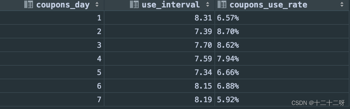

 Python

库包

1. pandas: 支持从CSV、JSON、SQL、Microsoft Excel load数据，可以对各种维度的数据做归并、再成形、选择，还有数据清洗和数据加工特征
2. numpy：存储和操作矩阵、数组计算的包：数组计算、逻辑运算、傅立叶变化和图形操作、跟线性代数相关的操作
3. Matplotlib：绘图工具可以绘制线图、散点图、等高线图、条形图、柱状图、3D 图形、甚至是图形动画等。
4. sklearn：它涵盖了分类、回归、聚类、降维、模型选择、数据预处理六大模块，降低机器学习实践门槛，将复杂的数学计算集成为简单的函数，并提供了众多公开数据集和学习案例。

import pandas as pd
import numpy as np
import matplotlib.pyplot as plt
from pylab import *
import seaborn as sns
 
from sklearn import model_selection, preprocessing, naive_bayes, metrics, svm
from sklearn.model_selection import train_test_split, GridSearchCV
from sklearn.linear_model import LogisticRegression
from sklearn.neighbors import KNeighborsClassifier
from sklearn import ensemble, tree
 
# 忽略警告提示
import warnings
warnings.filterwarnings('ignore')

1.导入和了解数据特征

data = pd.read_csv(r"/Users/xll/Documents/服务数据质量/测试数据1.csv")

#设置python中dataframe的print结果不带省略号
pd.set_option('display.max_columns',5, 'display.max_rows', 100)


#返回数据集行和列的元组，其中data.shape[0]代表返回行数，data.shape[1] 代表返回列数
print(data.shape) 

#返回数据集的所有列名
data.columns

#随机返回样本5行
data.sample(5)

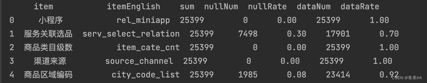
#返回前5行
print(data.head(5))

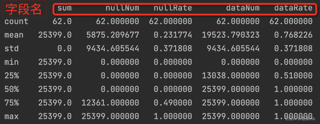
#返回浮点型和正行字段的均值、最大值、等统计数据
print(data.describe())

#numpy包的这个方法也是可以得到同样的结果
import numpy as np
print(data.describe(include=[np.number]))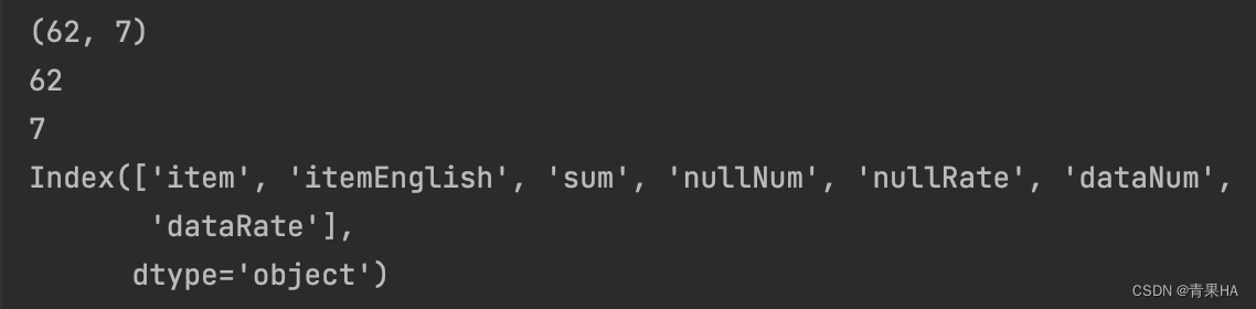

2.数据预处理:以泰坦尼克号沉船数据分析

2.1 读取数据，并随机获取5行观察数据特征

data = pd.read_csv('titanic.csv')
print(data.shape)  #输出：(891, 15)
data.sample(5)

2.2 查看各字段的缺失值

data.isnull().sum()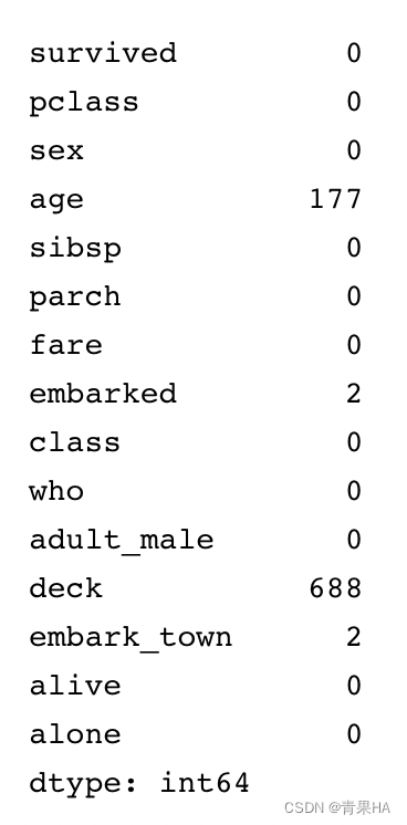

2.3 缺失值分析和缺失值处理

age、deck、embarked、embark_town 存在缺失值，需要处理。

（1）age 对生存率有影响，不能忽略，用平均值填充；

（2）总共有 891 条信息，deck 有 688 个缺失值，因此剔除 deck 这个分类标签；

（3）embarked、embark_town 缺失值较少，都为 2 个，随机取其中一个数据填充。

//用平均年龄补充年龄缺失的字段
data['age']=data['age'].fillna(data['age'].median())

//因该特征缺失占比是99%，所以删除deck特征
del data['deck']

//只有两条记录缺失，随机补充
data['embarked']=data['embarked'].fillna('S')
data['embark_town']=data['embark_town'].fillna('Southampton')
 
//再次查询下空值的记录总和，返回都是0
data.isnull().sum()

3.数据特征分析

3.1.1全体成员生存和死亡情况汇总

//定义一个survive的矩阵：死亡为0，生存为1；统计死亡人数、生存人数和死亡及生存率

survived = data['survived'].value_counts().to_frame().reset_index().rename(columns={'index': 'label', 'survived': 'counts'})
 
#计算存活率
survived_rate = round(342/891, 2)
survived['rate'] = [1-survived_rate, survived_rate]
print(survived)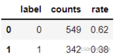

3.1.2绘制扇形图

mpl.rcParams['axes.unicode_minus'] = False     #处理无法显示中文的问题
mpl.rcParams['font.sans-serif'] = ['SimHei']  
 
fig=plt.figure(1,figsize=(6,6))
ax1=fig.add_subplot(1,1,1)  
label=['遇难','存活']
color=['#C23531','#F5DEB3']
explode=0.05,0.05  #扇区间隔
 
patches,l_text,p_text = ax1.pie(survived.rate,labels=label,colors=color,startangle=90,autopct='%1.0f%%',explode=explode,shadow=True)
for t in l_text:
    t.set_size(20)
for t in p_text:
    t.set_size(20)
ax1.set_title('全体成员的生存情况', fontsize=20)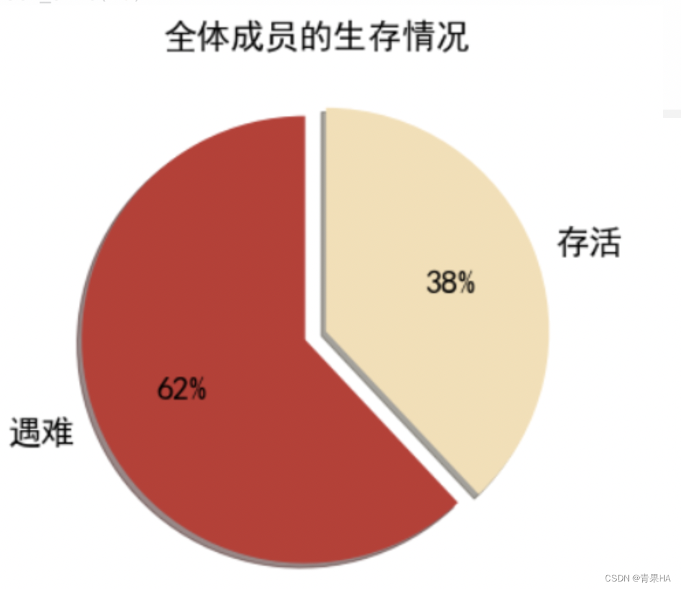 

3.1.3 其他特征数据分析

fig = plt.figure(figsize=(15,10))
fig.set(alpha=0.3)  # 设定图表颜色alpha参数(透明度)
 
plt.subplot2grid((2,3),(0,0))
data.survived.value_counts().plot(kind='bar')
plt.title("获救情况 (1为获救)")
plt.ylabel("人数")
 
plt.subplot2grid((2,3),(0,1))
data.pclass.value_counts().plot(kind="bar")
plt.ylabel("人数")
plt.title("乘客等级分布")
 
plt.subplot2grid((2,3),(0,2))
plt.scatter(data.survived, data.age)
plt.ylabel("年龄")
plt.grid(b=True, which='major', axis='y')
plt.title("按年龄看获救分布 (1为获救)")
 
plt.subplot2grid((2,3),(1,0), colspan=2)
data.age[data.pclass == 1].plot(kind='kde')
data.age[data.pclass == 2].plot(kind='kde')
data.age[data.pclass == 3].plot(kind='kde')
plt.xlabel("年龄")
plt.ylabel("密度")
plt.title("各等级的乘客年龄分布")
plt.legend(('头等舱', '2等舱','3等舱'),loc='best')
 
plt.subplot2grid((2,3),(1,2))
data.embarked.value_counts().plot(kind='bar')
plt.title("各登船口岸上船人数")
plt.ylabel("人数")
plt.show()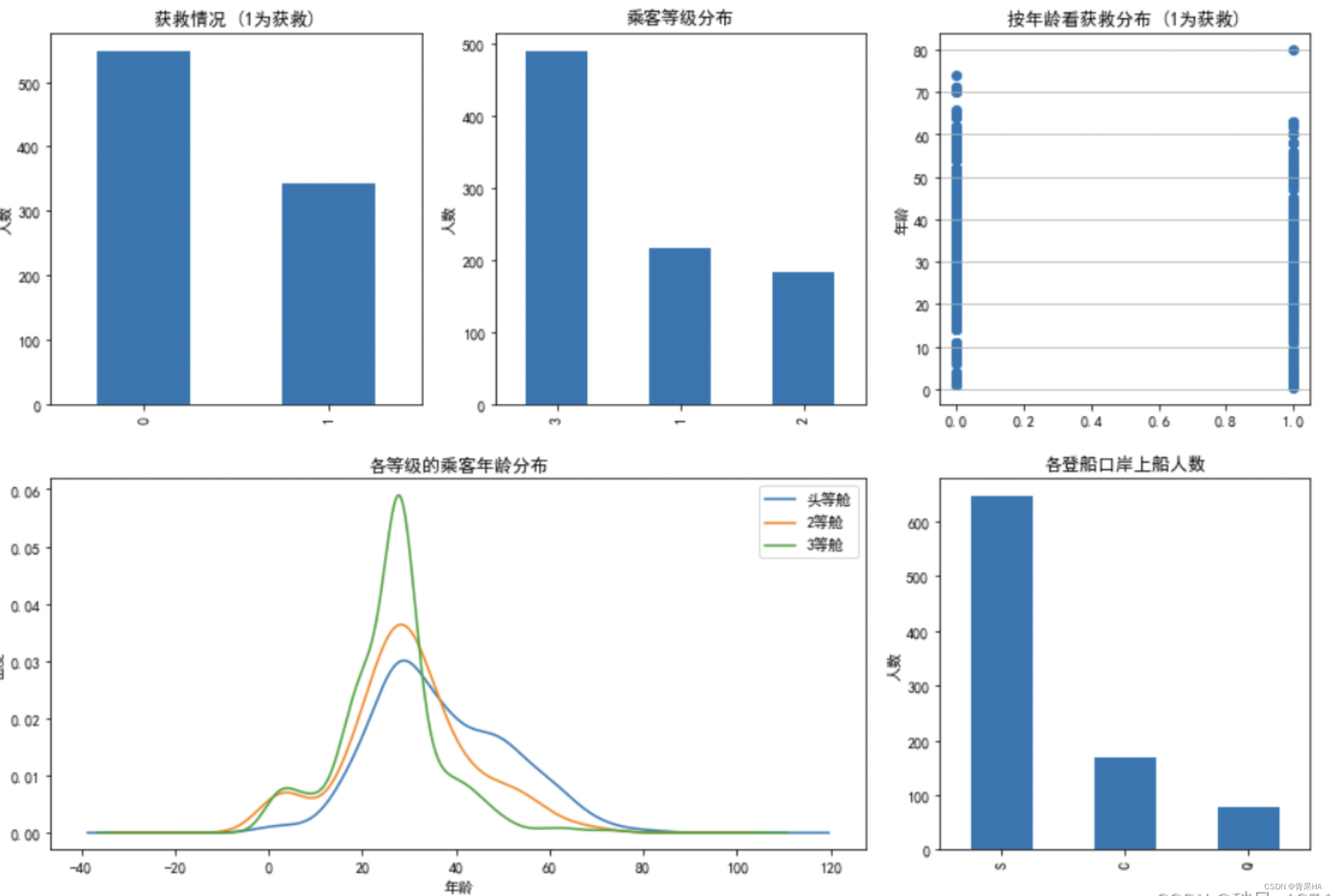

3.1.4 连续值特征（年龄、船票费用）对生存结果的影响

fig = plt.figure(figsize=(15,4))
 
plt.subplot2grid((2,2),(0,0))
data.age[data.survived == 0].plot(kind='box', vert=False, patch_artist=True, notch = True, color='#C23531', fontsize=15)
plt.grid(linestyle="--", alpha=0.8)
plt.title("遇难", fontsize=15)
 
plt.subplot2grid((2,2),(0,1))
data.fare[data.survived == 0].plot(kind='box', vert=False, patch_artist=True, notch = True, color='#C23531', fontsize=15)
plt.grid(linestyle="--", alpha=0.8)
plt.title("遇难", fontsize=15)
 
plt.subplot2grid((2,2),(1,0))
data.age[data.survived == 1].plot(kind='box', vert=False, patch_artist=True, notch = True, color='#F5DEB3', fontsize=15)
plt.grid(linestyle="--", alpha=0.8)
plt.xlabel("存活", fontsize=15)
 
plt.subplot2grid((2,2),(1,1))
data.fare[data.survived == 1].plot(kind='box', vert=False, patch_artist=True, notch = True, color='#F5DEB3', fontsize=15)
plt.grid(linestyle="--", alpha=0.8)
plt.xlabel("存活", fontsize=15)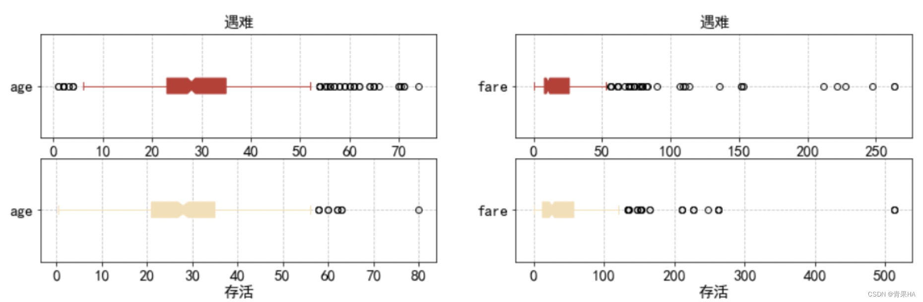

3.1.5 乘客等级、性别对生存结果的影响（从年龄的分布看）

mpl.rcParams.update({'font.size': 14})
fig,axes=plt.subplots(2,2,figsize=(18, 12))
sns.violinplot("pclass","age", hue="survived", data=data, palette='autumn',ax=axes[0][0]).set_title('Pclass and Age vs Survived')
sns.swarmplot(x="pclass", y="age",hue="survived", data=data,palette='autumn',ax=axes[1][0]).legend(loc='upper right').set_title('survived')
sns.violinplot("sex","age", hue="survived", data=data, palette='winter', ax=axes[0][1]).set_title('Sex and Age vs Survived')
sns.swarmplot(x="sex", y="age",hue="survived", data=data,palette='winter',ax=axes[1][1]).legend(loc='upper right').set_title('survived')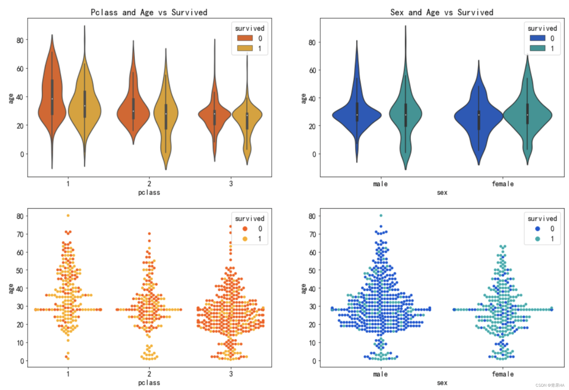

3.1.6 乘客等级、性别对生存结果的影响（从船票费用的分布看）

fig,axes=plt.subplots(2,2,figsize=(18, 12))
sns.violinplot("pclass","fare", hue="survived", data=data, palette='autumn',ax=axes[0][0]).set_title('Pclass and Age vs Survived')
sns.stripplot("pclass", "fare",hue="survived", data=data,palette='autumn',ax=axes[1][0]).legend(loc='upper right').set_title('survived')
sns.violinplot("sex","fare", hue="survived", data=data, palette='winter', ax=axes[0][1]).set_title('Sex and Age vs Survived')
sns.stripplot("sex", "fare",hue="survived", data=data,palette='winter',ax=axes[1][1]).legend(loc='upper right').set_title('survived')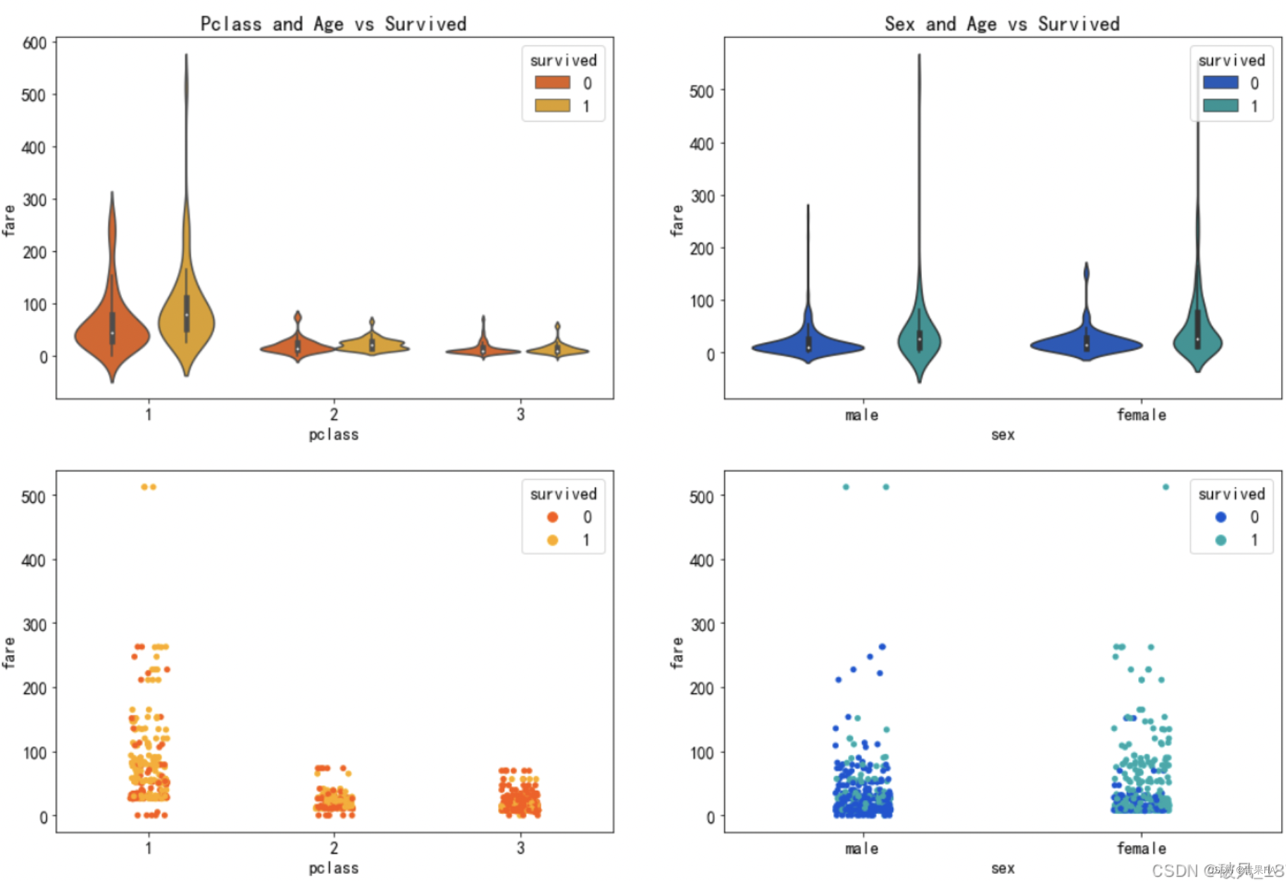

3.1.7 特征关联分析

sns.heatmap(data.corr(),annot=True,cmap='RdYlGn',linewidths=0.2)
fig=plt.gcf()
fig.set_size_inches(10,8)
plt.show()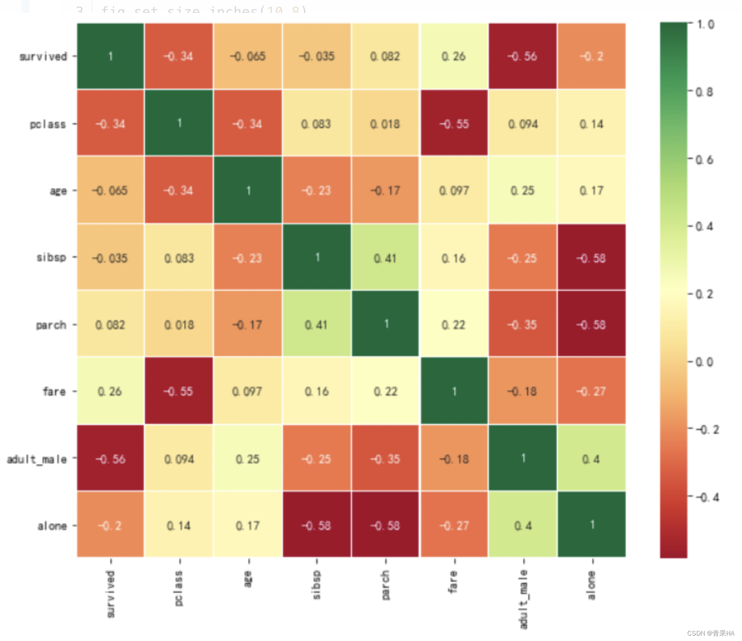

4.特征工程

4.1标签编码预处理

在所有标签中，survived 是分类标签，其余的 14 个变量是分类特征。 由于特征和标签的值存在非结构化类型，因此需要进行特征工程处理，即进行字符串编码处理。个人理解其实就是把非整型或浮点型的其他类型转化成整型

print(data.info())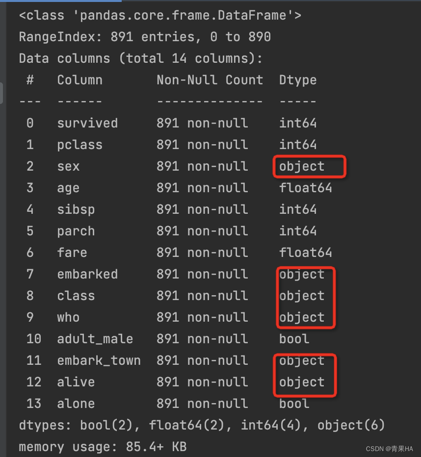

处理之前：前5行的数据是这样的 

print(data.head())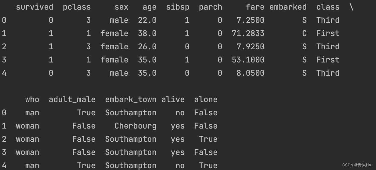

初始化编码器处理：处理之后的前5行，全部变成数值型 

le = preprocessing.LabelEncoder()
for col in data.columns:
    data[col] = le.fit_transform(data[col])
data.head()
data.to_csv('Preprocessing_Titanic.csv')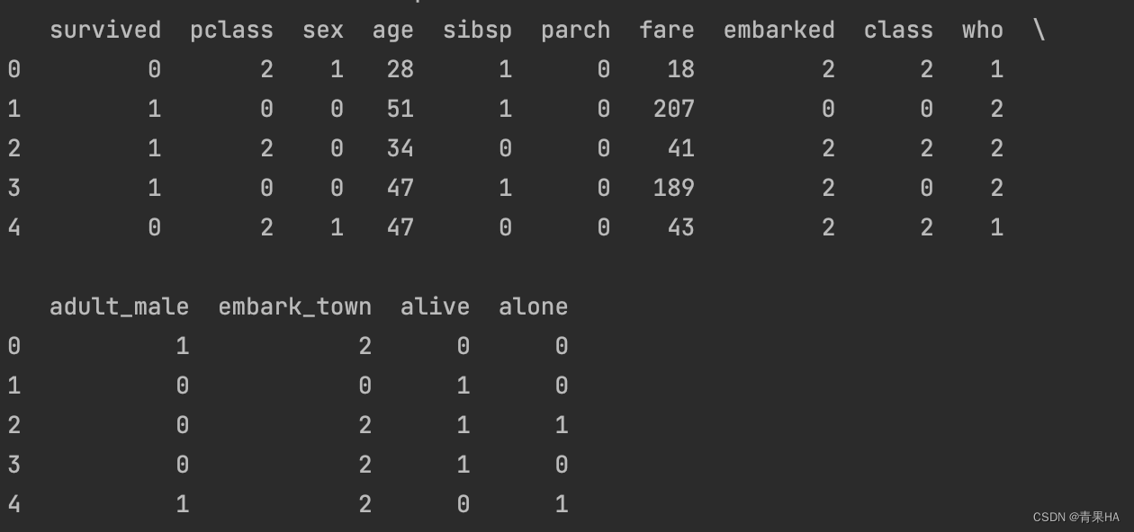

4.2 去除无意义的特征

名字对生存率几乎没有影响，所以删除 who 标签

del data['who']

4.3 去除同类重复的特征

eg:列1的性别：难，女和列2 的0，1，这个是基于在上一步编码处理成数值型之后；去除之后发现有三个重复的特征

data_ = data.T.drop_duplicates().T
print('去重前：', len(data.columns))
print('去重后：', len(data_.columns))
 
for a in data.columns:
    if a not in data_.columns:
        for b in data_.columns:
            if list(data[b].values) == list(data[a].values):
                print(f'重复标签: {a} 和 {b}')
data = data_


#drop_duplicates方法，它用于返回一个移除了重复行的DataFrame
#所以这里先做了转置的操作，剔除后，再转置回来的

#保留第一个重复行 data.drop_duplicates() 
#去除所有重复行 data.drop_duplicates(keep=False) 
#合并起来再去重，只剩下真的重复行 pd.concat([data0_1,data0_2]).drop_duplicates(keep=False)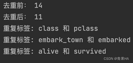

 4.4可视化探索各个特征的分布情况

result_plot = data.hist(bins=50, figsize=(14, 12))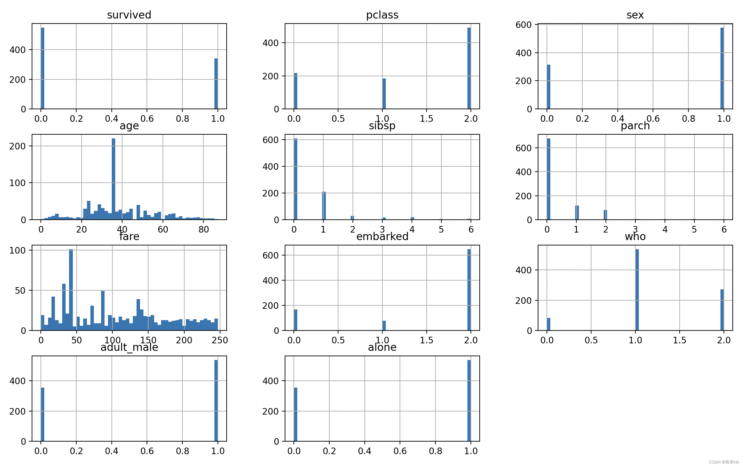

 由上面的可视化情况来看，不需要对特征进行标准化处理。

# 对数据进行标准化
# X = StandardScaler().fit_transform(X)

 5.模型训练

5.1  10折交叉验证分割数据集，9份做训练，1份做测试 ，确保训练和测试数据无交集

# data第一列是survived分类标签，作为y输出结果，其他类都是分类的特征，用于输入X
X = data.iloc[:, 1:]
y = data.iloc[:, 0]
 
x_train, x_test, y_train, y_test = train_test_split(X, y,test_size=0.1,shuffle=True,random_state=20)
 
print(x_train.shape)
print(x_test.shape)
print(y)
print(X)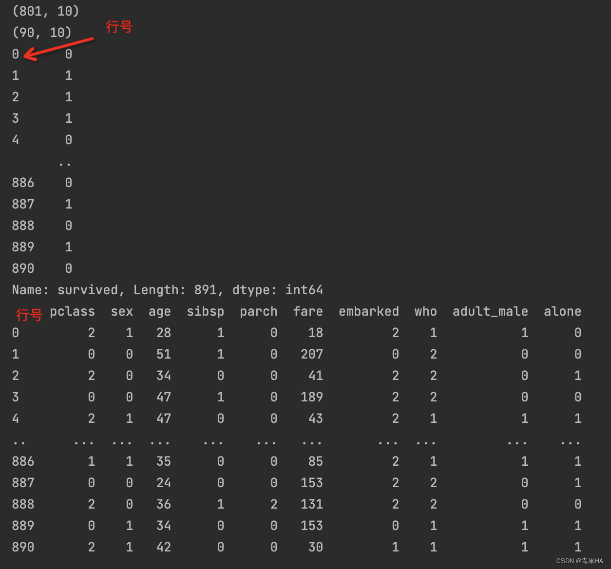

5.2. 建立模型训练及评估函数

 5.2.1建模：训练模型

model, train_score, test_score, roc_auc = [], [], [], []  # 存储相关模型信息，以便后续分析
 
def train_model(classifier, x_train, y_train, x_test):
    lr = classifier  # 初始化
    lr.fit(x_train, y_train)  # 训练
    y_pred_lr = lr.predict(x_test)  # 预测
 
    if '.' in str(classifier):
        model_name = str(classifier).split('(')[0].split('Classifier')[0].split('.')[1]
        print('\n{:=^60}'.format(model_name))
    else:
        model_name = str(classifier).split('(')[0].split('Classifier')[0]
        print('\n{:=^60}'.format(model_name))
    model.append(model_name)
        
    # 性能评估
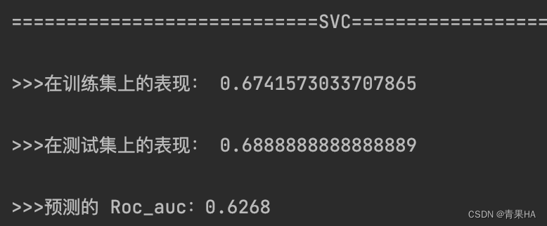
    print('\n>>>在训练集上的表现：', lr.score(x_train, y_train))
    print('\n>>>在测试集上的表现：', metrics.accuracy_score(y_test, y_pred_lr))
    print('\n>>>预测的 Roc_auc：%.4f' % metrics.roc_auc_score(y_test, y_pred_lr))
    print('\n>>>混淆矩阵'),show_confusion_matrix(metrics.confusion_matrix(y_test,y_pred_lr))
    
    train_score.append(lr.score(x_train, y_train))
    test_score.append(metrics.accuracy_score(y_test, y_pred_lr))
    roc_auc.append(metrics.roc_auc_score(y_test, y_pred_lr))

 5.2.2绘制分类矩阵函数

def show_confusion_matrix(cnf_matrix):
    plt.matshow(cnf_matrix,cmap=plt.cm.YlGn,alpha=0.7)
    ax=plt.gca()
    ax.set_xlabel('Predicted Label',fontsize=16)
    ax.set_xticks(range(0,len(survived.label)))
    ax.set_xticklabels(survived.label,rotation=45)
    ax.set_ylabel('Actual Label',fontsize=16,rotation=90)
    ax.set_yticks(range(0,len(survived.label)))
    ax.set_yticklabels(survived.label)
    ax.xaxis.set_label_position('top')
    ax.xaxis.tick_top()
    for row in range(len(cnf_matrix)):
        for col in range(len(cnf_matrix[row])):
            ax.text(col,row,cnf_matrix[row][col],va='center',ha='center',fontsize=16)
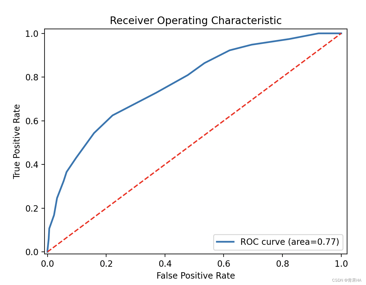
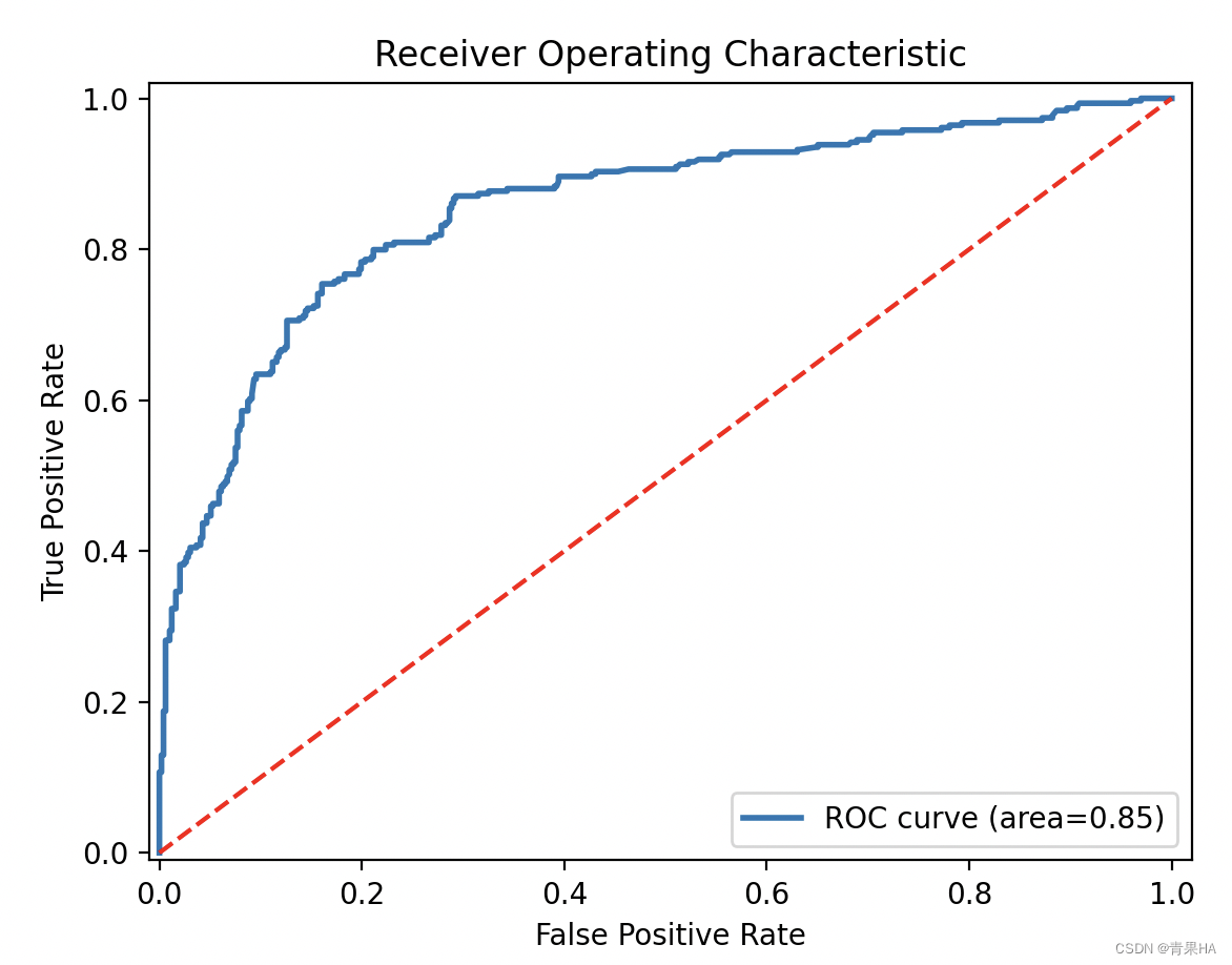
    plt.show()

5.2.3 绘制ROC曲线函数

def show_roc_line(classifier, x_train, y_train):  
    y_train_prob=classifier.predict_proba(x_train)
    y_pred_prob=y_train_prob[:,1]                             #正例率 
    fpr,tpr,thresholds=metrics.roc_curve(y_train,y_pred_prob) #计算ROC曲线
    auc=metrics.auc(fpr,tpr)                                  #计算AUC 
    plt.plot(fpr,tpr,lw=2,label='ROC curve (area={:.2f})'.format(auc))
    plt.plot([0,1],[0,1],'r--')
    plt.xlim([-0.01, 1.02])
    plt.ylim([-0.01, 1.02])
    plt.xlabel('False Positive Rate')
    plt.ylabel('True Positive Rate')
    plt.title('Receiver Operating Characteristic')
    plt.legend(loc='lower right')
    plt.show() 

6. 训练预测

6.1 决策树模型

classifier = tree.DecisionTreeClassifier()
train_model(classifier, x_train, y_train, x_test)  #建模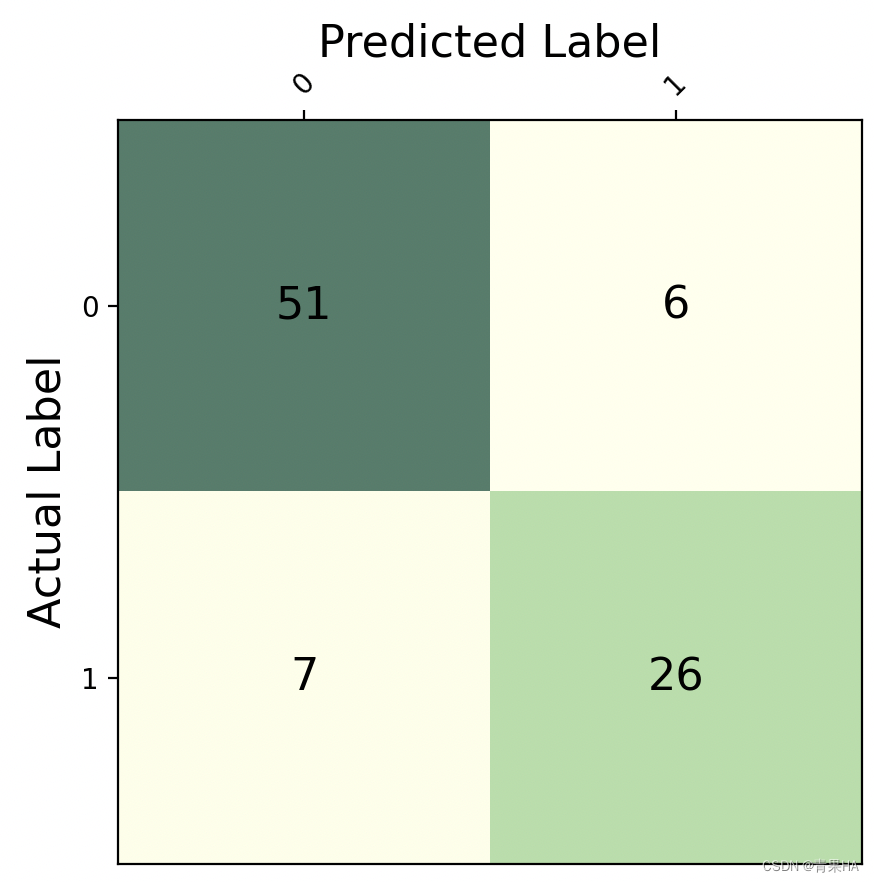

 绘制随机森林重要的特征

labels = X.columns
importances = classifier.feature_importances_  # 获取特征权重值
indices = np.argsort(importances)[::-1]  # 打印特征等级

features = [labels[i] for i in indices]
weights = [importances[i] for i in indices]

print("Feature ranking:")
for f in range(len(features)):
    print("%d. %s (%f)" % (f + 1, features[f], weights[f]))  # 绘制随机森林的特征重要性

plt.figure()
plt.title("Feature importances")
plt.bar(features, np.array(weights), color='r')
plt.xticks(rotation=90)
plt.title('Feature Weights')
plt.show()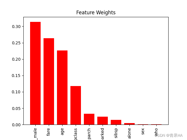

数据分析：从上面的可视化图可以看出，对生存率影响大的特征只有 4 个：fare(船票费用)、adult_male(成年男性)、age(年龄)、pclass(乘客等级)。

6.2KNN模型

classifier = KNeighborsClassifier(n_neighbors=20)
train_model(classifier, x_train, y_train, x_test)  
show_roc_line(classifier, x_train, y_train)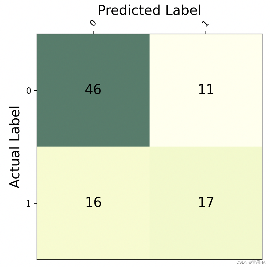

6.3 SVC模型

classifier = svm.SVC()
train_model(classifier, x_train, y_train, x_test)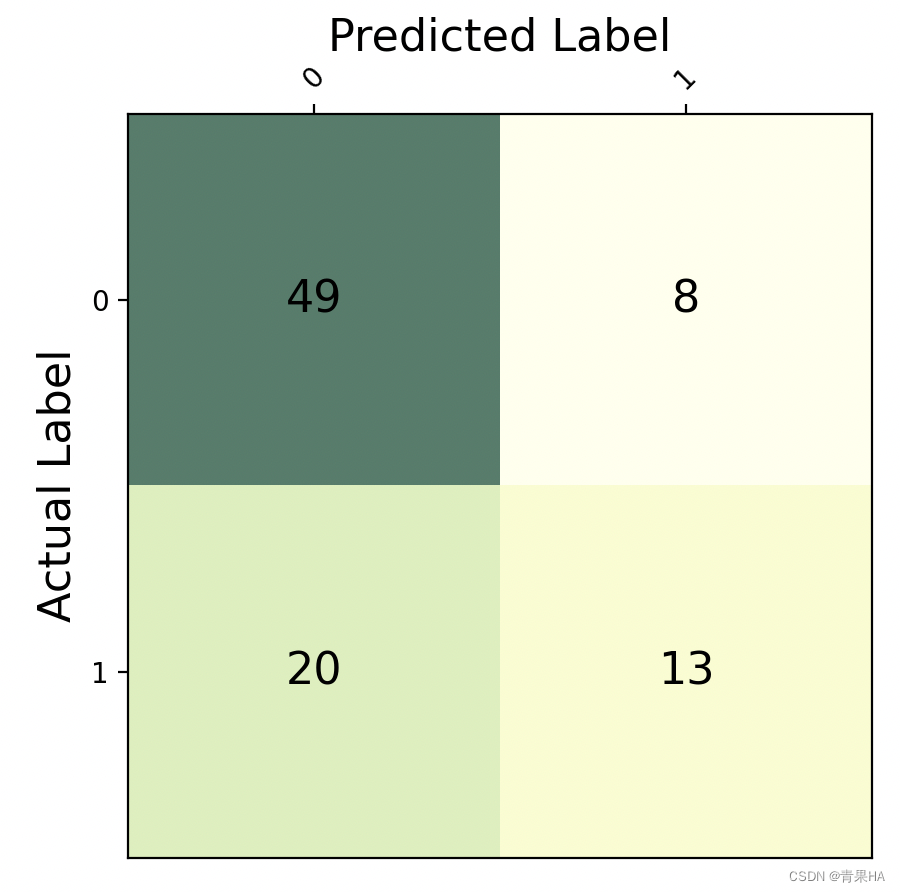

6.4 朴素贝叶斯

classifier = naive_bayes.GaussianNB()
train_model(classifier, x_train, y_train, x_test)  #建模

show_roc_line(classifier, x_train, y_train)  #绘制ROC曲线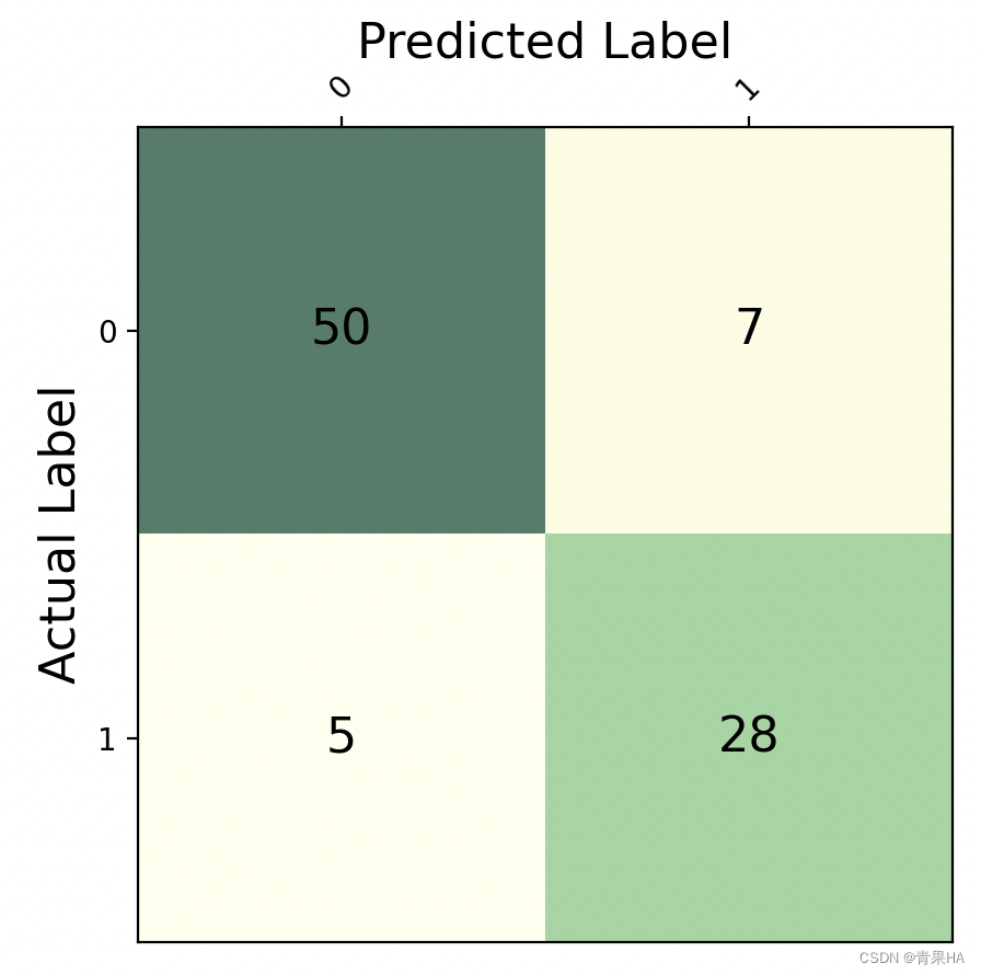

6.5 不同模型之间的准确率对比

df = pd.DataFrame()
df['model'] = model
df['Roc_auc'] = roc_auc
df['train_score'] = train_score
df['test_score'] = test_score
df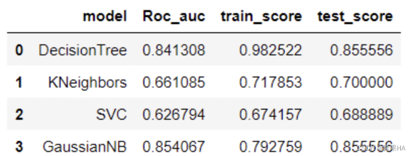

6.5.1结论：

评判标准：AUC(Area under Curve)ROC曲线以下的面积，介于0.1和1之间，其数值作为评判分类器好坏的标准时，值越大越好；

所以可以看出朴素贝叶斯分类预测效果更好，决策树在训练集上的表现较好，但在测试机表现一般，代表过拟合了

6.5.2 过拟合调参

param = [{'criterion':['gini'],'max_depth': np.arange(20,50,10),'min_samples_leaf':np.arange(2,8,2),
          'min_impurity_decrease':np.linspace(0.1,0.9,10)},
         {'criterion':['gini','entropy']},
         {'min_impurity_decrease':np.linspace(0.1,0.9,10)}]
clf = GridSearchCV(tree.DecisionTreeClassifier(),param_grid=param,cv=10)
clf.fit(x_train,y_train)
print('最优参数:', clf.best_params_)
print('最好成绩:', clf.best_score_)

6.5.3 用上述最优的参数生成决策树

model = tree.DecisionTreeClassifier(criterion= 'gini', max_depth=20, min_impurity_decrease=0.1, min_samples_leaf= 2)
model.fit(x_train, y_train)
y_pred = model.predict(x_test)
print('train score:', clf.score(x_train, y_train))
print('test score:', clf.score(x_test, y_test))
print("查准率：", metrics.precision_score(y_test,y_pred))
print('召回率:',metrics.recall_score(y_test,y_pred))
print('f1分数:', metrics.f1_score(y_test,y_pred)) #二分类评价标准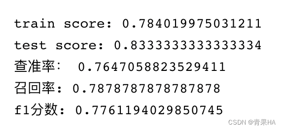

从结果来看，有所提升，但还是比朴素贝叶斯的预测分差一些

参考：

https://blog.csdn.net/twlve/article/details/128609147?spm=1001.2014.3001.5502

https://blog.csdn.net/twlve/article/details/128626526?spm=1001.2014.3001.5502

O2O优惠券核销-数据分析_十二十二呀的博客-CSDN博客_优惠券数据分析

https://blog.csdn.net/weixin_47068543/article/details/126151816