之前简单的利用深层自编码器对语音信号进行降噪
基于自编码器的语音信号降噪 – 哥廷根数学学派的文章 – 知乎 基于自编码器的语音信号降噪 – 知乎
本篇讲一些稍微复杂的基于深度学习的语音降噪方法,并比较了应用于同一任务的两种的网络:全连接层网络和卷积网络。
完整代码和数据集见如下链接
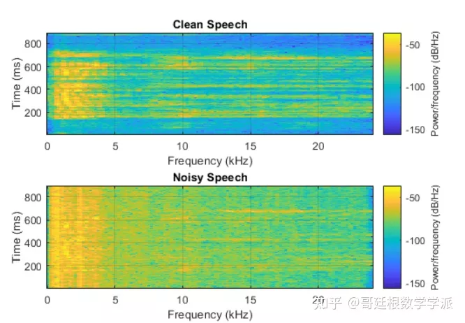
考虑以下以 8 kHz 采样的语音信号
[cleanAudio,fs] = audioread("SpeechDFT.wav");
sound(cleanAudio,fs)
将洗衣机噪声添加到上述的语音信号中,设置噪声功率,使信噪比 (SNR) 为0dB
noise = audioread("WashingMachine.mp3");接下来从噪声文件中的随机位置提取噪声段
ind = randi(numel(noise) - numel(cleanAudio) + 1, 1, 1);
noiseSegment = noise(ind:ind + numel(cleanAudio) - 1);
speechPower = sum(cleanAudio.^2);
noisePower = sum(noiseSegment.^2);
noisyAudio = cleanAudio + sqrt(speechPower/noisePower) * noiseSegment;
%播放信号
sound(noisyAudio,fs)
可视化原始信号和噪声信号
t = (1/fs) * (0:numel(cleanAudio)-1);
subplot(2,1,1)
plot(t,cleanAudio)
title("Clean Audio")
grid on
subplot(2,1,2)
plot(t,noisyAudio)
title("Noisy Audio")
xlabel("Time (s)")
grid on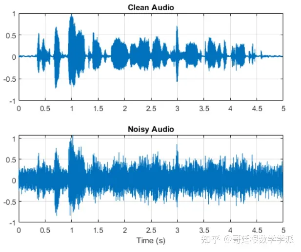
语音降噪的目的是从语音信号中去除洗衣机噪声,同时最大限度地减少输出语音信号中不希望的所谓的artifacts。
检查数据集
本例使用的数据集包含 48 kHz 的短句录音
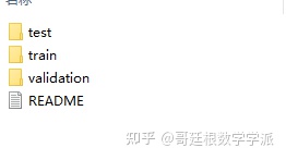
训练集,测试集,验证集文件
训练集部分数据
使用 audioDatastore 为训练集创建数据存储
adsTrain = audioDatastore(fullfile(dataFolder,'train'),'IncludeSubfolders',true);读取datastore中第一个文件的内容
[audio,adsTrainInfo] = read(adsTrain);播放语音信号
sound(audio,adsTrainInfo.SampleRate)绘制语音信号
figure
t = (1/adsTrainInfo.SampleRate) * (0:numel(audio)-1);
plot(t,audio)
title("Example Speech Signal")
xlabel("Time (s)")
grid on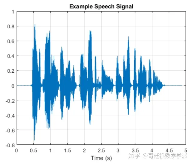
深度学习系统概述
基本的深度学习训练方案如下图所示。
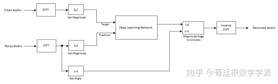
对于熟悉语音信号处理的同学肯定是小case。注意,由于语音通常低于 4 kHz,因此首先将干净和嘈杂的语音信号下采样到 8 kHz,以减少网络的计算负担。 网络的输出是降噪信号的幅度谱,使用输出幅度谱和噪声信号的相位将降噪后的音频转换回时域[1]。
可以使用短时傅里叶变换 (STFT) 将音频信号转换到频域,使用Hamming窗,窗口长度为 256 ,重叠率为 75%。Predicter的输入由 8 个连续的噪声 STFT 向量组成,因此每个 STFT 输出估计值都是基于当前的噪声 STFT 和 7 个先前的噪声 STFT 向量计算的。
如何从一个训练文件生成Target和Predicter(直接用英文单词了,否则容易引起误解)?首先,定义系统参数:
windowLength = 256;
win = hamming(windowLength,"periodic");
overlap = round(0.75 * windowLength);
ffTLength = windowLength;
inputFs = 48e3;
fs = 8e3;
numFeatures = ffTLength/2 + 1;
numSegments = 8;
创建一个 dsp.SampleRateConverter 对象以将 48 kHz 音频转换为 8 kHz,
src = dsp.SampleRateConverter("InputSampleRate",inputFs, ...
                              "OutputSampleRate",fs, ...
                              "Bandwidth",7920);
从datastore中读入音频文件的内容
audio = read(adsTrain);注意:要确保音频长度是采样率转换器抽取因子的倍数
decimationFactor = inputFs/fs;
L = floor(numel(audio)/decimationFactor);
audio = audio(1:decimationFactor*L);
将音频信号转换为 8 kHz
audio = src(audio);
reset(src)
从洗衣机噪声向量中创建一个随机噪声段
randind = randi(numel(noise) - numel(audio),[1 1]);
noiseSegment = noise(randind : randind + numel(audio) - 1);
向语音信号中添加噪声,使 SNR 为 0 dB。
noisePower = sum(noiseSegment.^2);
cleanPower = sum(audio.^2);
noiseSegment = noiseSegment .* sqrt(cleanPower/noisePower);
noisyAudio = audio + noiseSegment;
使用STFT从原始和嘈杂的音频信号生成幅值STFT向量
cleanSTFT = stft(audio,'Window',win,'OverlapLength',overlap,'FFTLength',ffTLength);
cleanSTFT = abs(cleanSTFT(numFeatures-1:end,:));
noisySTFT = stft(noisyAudio,'Window',win,'OverlapLength',overlap,'FFTLength',ffTLength);
noisySTFT = abs(noisySTFT(numFeatures-1:end,:));
从嘈杂的 STFT 生成 8 段训练Predicter信号,对应深度学习训练方案图
noisySTFT = [noisySTFT(:,1:numSegments - 1), noisySTFT];
stftSegments = zeros(numFeatures, numSegments , size(noisySTFT,2) - numSegments + 1);
for index = 1:size(noisySTFT,2) - numSegments + 1
stftSegments(:,:,index) = (noisySTFT(:,index:index + numSegments - 1));
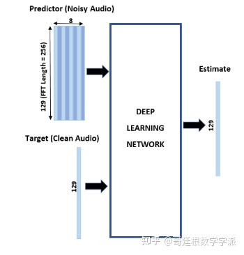
end设置Target和Predicter,每个Predicter维度为 129×8,每个Target为 129×1,这些都是可以根据信号调整的
targets = cleanSTFT;
size(targets)
predictors = stftSegments;
size(predictors)
为了加快处理速度,使用 tall 数组从datastore中所有音频文件的语音片段中提取特征序列,要是有matlab的并行工具箱和GPU。
首先,将datastore转换为 tall 数组,此处需要的时间较长
reset(adsTrain)
T = tall(adsTrain)
从 tall 表中提取Target和Predicter的幅值STFT,这一步很重要,GenerateSpeechDenoisingFeatures是提取Target和Predicter的幅值STFT的函数,我还需要优化一点
[targets,predictors] = cellfun(@(x)GenerateSpeechDenoisingFeatures(x,noise,src),T,"UniformOutput",false);

[targets,predictors] = gather(targets,predictors);
将所有特征进行归一化,分别计算Target和Predicter的均值和标准差,并使用它们对数据进行归一化。
predictors = cat(3,predictors{:});
noisyMean = mean(predictors(:));
noisyStd = std(predictors(:));
predictors(:) = (predictors(:) - noisyMean)/noisyStd;
targets = cat(2,targets{:});
cleanMean = mean(targets(:));
cleanStd = std(targets(:));
targets(:) = (targets(:) - cleanMean)/cleanStd;
将Target和Predicter进行维度重塑,即reshape为与深度学习网络相对应的维度
predictors = reshape(predictors,size(predictors,1),size(predictors,2),1,size(predictors,3));
targets = reshape(targets,1,1,size(targets,1),size(targets,2));
将数据随机分成训练集和验证集。
inds = randperm(size(predictors,4));
L = round(0.99 * size(predictors,4));

trainPredictors = predictors(:,:,:,inds(1:L));
trainTargets = targets(:,:,:,inds(1:L));

validatePredictors = predictors(:,:,:,inds(L+1:end));
validateTargets = targets(:,:,:,inds(L+1:end));
下面开始步入正题,进行第一个全连接层深层网络的语音降噪
全连接网络是什么就不讲了,看图
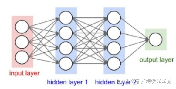
定义网络层,将输入大小指定为大小为 NumFeatures-by-NumSegments(本例中为 129-by-8)的图像。 定义两个隐藏的全连接层,每个层有 1024 个神经元。 由于是纯线性系统,因此在每个隐藏的全连接层之后都有一个整流线性单元 (ReLU) 层。 批量归一化层对输出的均值和标准差进行归一化,添加一个具有 129 个神经元的全连接层,然后是一个回归层。
layers = [
    imageInputLayer([numFeatures,numSegments])
    fullyConnectedLayer(1024)
    batchNormalizationLayer
    reluLayer
    fullyConnectedLayer(1024)
    batchNormalizationLayer
    reluLayer
    fullyConnectedLayer(numFeatures)
    regressionLayer
    ];
然后设置网络的训练选项,很好理解
miniBatchSize = 128;
options = trainingOptions("adam", ...
    "MaxEpochs",3, ...
    "InitialLearnRate",1e-5,...
    "MiniBatchSize",miniBatchSize, ...
    "Shuffle","every-epoch", ...
    "Plots","training-progress", ...
    "Verbose",false, ...
    "ValidationFrequency",floor(size(trainPredictors,4)/miniBatchSize), ...
    "LearnRateSchedule","piecewise", ...
    "LearnRateDropFactor",0.9, ...
    "LearnRateDropPeriod",1, ...
    "ValidationData",{validatePredictors,validateTargets});
利用trainNetwork 使用指定的训练选项和网络层训练深层网络。 因为训练集很大,训练过程较为耗时
denoiseNetFullyConnected = trainNetwork(trainPredictors,trainTargets,layers,options);计算网络全连接层的权重数量
numWeights = 0;
for index = 1:numel(denoiseNetFullyConnected.Layers)
    if isa(denoiseNetFullyConnected.Layers(index),"nnet.cnn.layer.FullyConnectedLayer")
        numWeights = numWeights + numel(denoiseNetFullyConnected.Layers(index).Weights);
    end
end
fprintf("The number of weights is %d.\n",numWeights);
然后进行卷积层神经网络的语音去噪
卷积层通常比全连接层包含更少的参数,根据文献[2]中描述的全卷积网络的层数,包括 16 个卷积层。 前 15 个卷积层为3层的组,重复 5 次,滤波器宽度分别为 9、5 和 9,滤波器数量分别为 18、30 和 8。 最后一个卷积层的滤波器宽度为129 。 在这个网络中,卷积只在一个方向(沿着频率维度)执行,并且除了第一层之外的所有层,沿着时间维度的滤波器宽度设置为 1。 与全连接网络类似,卷积层之后是 ReLu 和批量归一化层。
layers = [imageInputLayer([numFeatures,numSegments])
          convolution2dLayer([9 8],18,"Stride",[1 100],"Padding","same")
          batchNormalizationLayer
          reluLayer

          repmat( ...
          [convolution2dLayer([5 1],30,"Stride",[1 100],"Padding","same")
          batchNormalizationLayer
          reluLayer
          convolution2dLayer([9 1],8,"Stride",[1 100],"Padding","same")
          batchNormalizationLayer
          reluLayer
          convolution2dLayer([9 1],18,"Stride",[1 100],"Padding","same")
          batchNormalizationLayer
          reluLayer],4,1)

          convolution2dLayer([5 1],30,"Stride",[1 100],"Padding","same")
          batchNormalizationLayer
          reluLayer
          convolution2dLayer([9 1],8,"Stride",[1 100],"Padding","same")
          batchNormalizationLayer
          reluLayer

          convolution2dLayer([129 1],1,"Stride",[1 100],"Padding","same")

          regressionLayer
          ];
训练选项与全连接网络的选项类似
options = trainingOptions("adam", ...
    "MaxEpochs",3, ...
    "InitialLearnRate",1e-5, ...
    "MiniBatchSize",miniBatchSize, ...
    "Shuffle","every-epoch", ...
    "Plots","training-progress", ...
    "Verbose",false, ...
    "ValidationFrequency",floor(size(trainPredictors,4)/miniBatchSize), ...
    "LearnRateSchedule","piecewise", ...
    "LearnRateDropFactor",0.9, ...
    "LearnRateDropPeriod",1, ...
    "ValidationData",{validatePredictors,permute(validateTargets,[3 1 2 4])});
利用 trainNetwork 使用指定的训练选项和层架构训练网络
denoiseNetFullyConvolutional = trainNetwork(trainPredictors,permute(trainTargets,[3 1 2 4]),layers,options);计算网络全连接层的权重数量
numWeights = 0;
for index = 1:numel(denoiseNetFullyConvolutional.Layers)
    if isa(denoiseNetFullyConvolutional.Layers(index),"nnet.cnn.layer.Convolution2DLayer")
        numWeights = numWeights + numel(denoiseNetFullyConvolutional.Layers(index).Weights);
    end
end
fprintf("The number of weights in convolutional layers is %d\n",numWeights);
测试降噪网络
读入测试集
adsTest = audioDatastore(fullfile(dataFolder,'test'),'IncludeSubfolders',true);从datastore中读取文件
[cleanAudio,adsTestInfo] = read(adsTest);确保音频长度是采样率转换器抽取因子的倍数
L = floor(numel(cleanAudio)/decimationFactor);
cleanAudio = cleanAudio(1:decimationFactor*L);
将音频信号转换为 8 kHz。
cleanAudio = src(cleanAudio);
reset(src)
测试阶段使用训练阶段未使用的洗衣机噪声来给语音信号加噪
noise = audioread("WashingMachine-16-8-mono-200secs.mp3");从洗衣机噪声向量中创建一个随机噪声段
randind = randi(numel(noise) - numel(cleanAudio), [1 1]);
noiseSegment = noise(randind : randind + numel(cleanAudio) - 1);
向语音信号中添加噪声,使 SNR为0 dB
noisePower = sum(noiseSegment.^2);
cleanPower = sum(cleanAudio.^2);
noiseSegment = noiseSegment .* sqrt(cleanPower/noisePower);
noisyAudio = cleanAudio + noiseSegment;
同样使用STFT从嘈杂的语音信号中生成幅值STFT向量
noisySTFT = stft(noisyAudio,'Window',win,'OverlapLength',overlap,'FFTLength',ffTLength);
noisyPhase = angle(noisySTFT(numFeatures-1:end,:));
noisySTFT = abs(noisySTFT(numFeatures-1:end,:));
同样从STFT 生成 8 段训练Predicter信号
noisySTFT = [noisySTFT(:,1:numSegments-1) noisySTFT];
predictors = zeros( numFeatures, numSegments , size(noisySTFT,2) - numSegments + 1);
for index = 1:(size(noisySTFT,2) - numSegments + 1)
    predictors(:,:,index) = noisySTFT(:,index:index + numSegments - 1);
end
通过在训练阶段计算的均值和标准差对Predicter进行归一化。
predictors(:) = (predictors(:) - noisyMean) / noisyStd;通过对两个经过训练的网络计算降噪幅值STFT
predictors = reshape(predictors, [numFeatures,numSegments,1,size(predictors,3)]);
STFTFullyConnected = predict(denoiseNetFullyConnected, predictors);
STFTFullyConvolutional = predict(denoiseNetFullyConvolutional, predictors);
通过训练阶段使用的平均值和标准差来恢复输出
STFTFullyConnected(:) = cleanStd * STFTFullyConnected(:) + cleanMean;
STFTFullyConvolutional(:) = cleanStd * STFTFullyConvolutional(:) + cleanMean;
将单边STFT 转换为“居中的” STFT,这在信号处理中很好理解
STFTFullyConnected = STFTFullyConnected.' .* exp(1j*noisyPhase);
STFTFullyConnected = [conj(STFTFullyConnected(end-1:-1:2,:)); STFTFullyConnected];
STFTFullyConvolutional = squeeze(STFTFullyConvolutional) .* exp(1j*noisyPhase);
STFTFullyConvolutional = [conj(STFTFullyConvolutional(end-1:-1:2,:)) ; STFTFullyConvolutional];
计算降噪语音信号。 istft 执行逆 STFT,使用带噪声STFT相位的相位来重建时域信号
denoisedAudioFullyConnected = istft(STFTFullyConnected,  ...
                                    'Window',win,'OverlapLength',overlap, ...
                                    'FFTLength',ffTLength,'ConjugateSymmetric',true);

denoisedAudioFullyConvolutional = istft(STFTFullyConvolutional,  ...
                                        'Window',win,'OverlapLength',overlap, ...
                                        'FFTLength',ffTLength,'ConjugateSymmetric',true);
绘制干净、嘈杂和降噪后的音频信号
t = (1/fs) * (0:numel(denoisedAudioFullyConnected)-1);

figure

subplot(4,1,1)
plot(t,cleanAudio(1:numel(denoisedAudioFullyConnected)))
title("Clean Speech")
grid on

subplot(4,1,2)
plot(t,noisyAudio(1:numel(denoisedAudioFullyConnected)))
title("Noisy Speech")
grid on

subplot(4,1,3)
plot(t,denoisedAudioFullyConnected)
title("Denoised Speech (Fully Connected Layers)")
grid on

subplot(4,1,4)
plot(t,denoisedAudioFullyConvolutional)
title("Denoised Speech (Convolutional Layers)")
grid on
xlabel("Time (s)")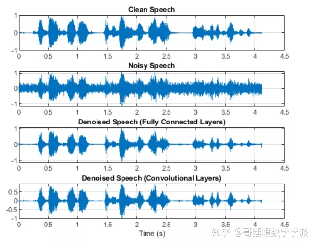
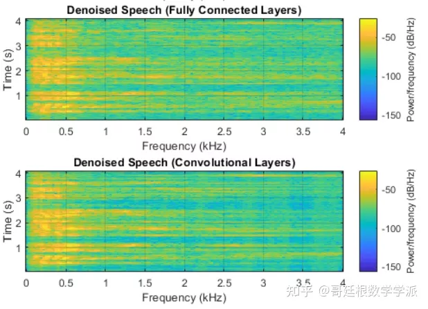
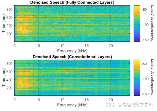
绘制干净、嘈杂和降噪后的频谱图。
h = figure;

subplot(4,1,1)
spectrogram(cleanAudio,win,overlap,ffTLength,fs);
title("Clean Speech")
grid on

subplot(4,1,2)
spectrogram(noisyAudio,win,overlap,ffTLength,fs);
title("Noisy Speech")
grid on

subplot(4,1,3)
spectrogram(denoisedAudioFullyConnected,win,overlap,ffTLength,fs);
title("Denoised Speech (Fully Connected Layers)")
grid on

subplot(4,1,4)
spectrogram(denoisedAudioFullyConvolutional,win,overlap,ffTLength,fs);
title("Denoised Speech (Convolutional Layers)")
grid on

p = get(h,'Position');
set(h,'Position',[p(1) 65 p(3) 800]);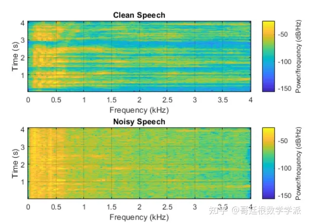
sound(noisyAudio,fs)播放全连接层神经网络降噪后的语音信号
sound(denoisedAudioFullyConnected,fs)播放卷积层神经网络降噪后的语音信号
sound(denoisedAudioFullyConvolutional,fs)播放干净的语音信号
sound(cleanAudio,fs)测试更多文件,且生成时域图和频域图,同时返回干净、加噪和降噪后的语音信号
[cleanAudio,noisyAudio,denoisedAudioFullyConnected,denoisedAudioFullyConvolutional] = testDenoisingNets(adsTest,denoiseNetFullyConnected,denoiseNetFullyConvolutional,noisyMean,noisyStd,cleanMean,cleanStd);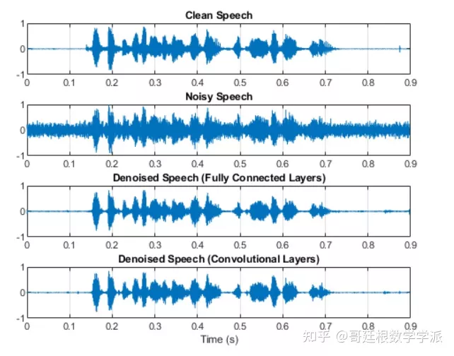
训练非常耗时,必须要配备matlab并行工具箱和GPU
另外,此方法可迁移至其他的一维信号,比如微震信号,机械振动信号,心电信号等,但要特别注意所加噪声信号的相位问题。
参考文献
[1] "Experiments on Deep Learning for Speech Denoising", Ding Liu, Paris Smaragdis, Minje Kim, INTERSPEECH, 2014.
[2] "A Fully Convolutional Neural Network for Speech Enhancement", Se Rim Park, Jin Won Lee, INTERSPEECH, 2017.
文章出处登录后可见!