内容

一、数据说明

(1) 数据的获取

(2) 数据预处理与分析

2.初步回归分析

(1) 模型和变量

(2) 参数估计

(3) 假设检验

1. 回归显著性检验

2. 回归系数的显著性检验

3. 回归子集的显著性检验

3.变量选择

(1) 最优子集选择

(2) 逐步回归

(3) 最终模型

(4) 假设检验

1. 回归显著性检验

2. 回归系数的显著性检验

(6) 残差分析

4.多重共线性

(1) 诊断

1. 相关系数

2. 方差膨胀因子(VIF)

3. 特征系统分析

(2) 主成分回归

1. 主成分分析

2. 主成分回归

(3) 岭回归

五、模型效果及结果分析

(1) 训练集

(2) 测试集

一、数据说明

(1) 数据的获取

本文选取2020年6月1日到2021年9月30日之间顺丰控股股票的相关数据作为训练集、2021年10月8日到2021年12月17日的顺丰控股股票的相关数据作为测试集，其中指标为交易日期(trade_date)、股票代码(ts_code)、开盘价(open)、最高价(high)、最低价(low)、收盘价(close)、前一日收盘价(pre_close)、涨跌额(change)、涨跌幅(pct_chg)、成交量(vol)、成交额(amount)及换手率(turnover_rate)。以上均通过tushare网站（个人ID：411335）的数据接口运用python获取：

import tushare as ts
import pandas as pd

ts.set_token('Your Token') # 输入个人Tushare接口
pro=ts.pro_api()

df1 = ts.pro_bar(ts_code='002352.SZ', adj='qfq', start_date='20200601', end_date='20210930',factors=['tor'])
df1 = df1[::-1]
df1.to_csv("data_train.csv")

df2 = ts.pro_bar(ts_code='002352.SZ', adj='qfq', start_date='20211008', end_date='20211217',factors=['tor'])
df2 = df2[::-1]
df2.to_csv("data_test.csv")

(2) 数据预处理与分析

首先，本文对原始数据进行过滤，保留研究所需的数据，去除冗余和缺失的数据。然后，由于本文对前一天的数据对第二天股价的影响感兴趣，因此将第二天的开盘价和收盘价添加到数据集中。最后，由于数据量大，解释变量存在差异，本文对其进行了标准化：

# 训练集
train.org = read.csv("data_train.csv")[,-1] 
train.org$trade_date = as.Date(as.character(train.org[,1]),format="%Y%m%d")

library(dplyr)
train.need = dplyr::select(train.org, open:close, amount, turnover_rate) # 数据筛选

train.Y = train.need$close[-1]
train.X = train.need[-dim(train.need)[1], ]
X.next_open = train.need$open[-1]

train.data = cbind(train.X, next_open = X.next_open, next_close = train.Y) # 最终数据
train.scale = data.frame(scale(train.data)) # 标准化数据
head(train.scale)

# 测试集
test.org = read.csv("data_test.csv")[,-1]
test.org$trade_date = as.Date(as.character(test.org[,1]),format="%Y%m%d")

test.need = dplyr::select(test.org, open:close, amount, turnover_rate)

test.Y = test.need$close[-1]
test.X = test.need[-dim(test.need)[1], ]
X.next_open = test.need$open[-1]

test.data = cbind(test.X, next_open = X.next_open, next_close = test.Y)
test.scale = data.frame(scale(test.data))
head(test.scale)

对训练集数据做初步的描述性统计，方便后续分析：

library(ggplot2)
library(ggthemes)

# 后一日收盘价走势
p1 = ggplot(train.org) + geom_line(aes(x=trade_date, y=close), lwd=1, col="darkblue") + labs(x="Trade Date",y = "Close Price (RMB)") + theme_economist() + theme(axis.title = element_text(face = "bold"))
p1

# 每日收益情况
p2 = train.org %>% mutate(bd=ifelse(pct_chg>=0, ">=0", "<0")) %>% ggplot(aes(x=bd)) + geom_bar(fill=c("green4", "red3"), width=0.3) + labs(x="Profit", y="Count")
p2

# 每日涨跌额分布情况
p3 = ggplot(train.org) + geom_density(aes(x=change,colour=I("royalblue")), lwd=1)+
  labs(x="Difference",y = "Density")
p3

输出：

图1 后一日收盘价走势图

图2 每日收益情况

图3 每日涨跌额分布曲线

可以看出，训练集中的数据涨跌次数基本一致，近似中心分布。

2.初步回归分析

(1) 模型和变量

初始模型为：

$y^\ast=\beta_1\ x_1^\ast+\beta_2\ x_2^\ast+\beta_3\ x_3^\ast+\beta_4\ x_4^\ast+\beta_5\ x_5^\ast+\beta_6\ x_6^\ast+\beta_7\ x_7^\ast+\varepsilon$

解释变量为标准化开盘价、最高价、最低价、收盘价、成交量、换手率、次日开盘价；响应变量是第二天的标准化收盘价。

(2) 参数估计

sol.lm1 = lm(next_close ~ .-1, train.scale)
summary(sol.lm1)

输出：

Call:
lm(formula = next_close ~ . - 1, data = train.scale)

Residuals:
     Min       1Q   Median       3Q      Max 
-0.50835 -0.07960 -0.01467  0.07265  0.59552 

Coefficients:
               Estimate Std. Error t value Pr(>|t|)    
open          -0.032552   0.121366  -0.268    0.789    
high           0.121204   0.147730   0.820    0.413    
low            0.051732   0.155783   0.332    0.740    
close          0.002069   0.155957   0.013    0.989    
amount        -0.009392   0.056105  -0.167    0.867    
turnover_rate  0.005953   0.049145   0.121    0.904    
next_open      0.853367   0.092863   9.190   <2e-16 ***
---
Signif. codes:  0 ‘***’ 0.001 ‘**’ 0.01 ‘*’ 0.05 ‘.’ 0.1 ‘ ’ 1

Residual standard error: 0.1314 on 317 degrees of freedom
Multiple R-squared:  0.983,	Adjusted R-squared:  0.9827 
F-statistic:  2626 on 7 and 317 DF,  p-value: < 2.2e-16

所以最小二乘估计的经验方程为：

$y\widehat\\^\ast\ =-0.0326x_1^\ast+0.1212x_2^\ast+0.0517x_3^\ast+0.0021x_4^\ast-0.0094x_5^\ast+0.0060x_6^\ast+0.8534x_7^\ast$

(3) 假设检验

1. 回归显著性检验

由上面结果可以得到检验统计量为2626，自由度为(7，317)，检验的p值约等于0，因此认为回归方程是显著的。

2. 回归系数的显著性检验

由上面结果可以看到，在0.05的显著性水平下，只有 $\beta_7\$ 是显著的。

3. 回归子集的显著性检验

由于前六个回归系数的显着性检验没有拒绝原假设，因此检验了由这六个变量组成的子集的显着性。比方说：

$H_0\ : A\theta=0\ \ vs\ \ H_1\ : A\theta\neq0$

其中， $A=(I_6,\ 0_6,_1\ ),\ \theta=(\beta_1,\beta_2,\beta_3,\beta_4,\beta_5,\beta_6)\prime$ 。

beta_set = result$coefficients[-1,1]
X_set = train.scale[,c(-1,-8)]
X = train.scale[,1]
NX = diag(1, dim(train.scale)[1]) - X%*%solve(t(X)%*%X)%*%X # 正交投影矩阵
fz = t(beta_set)%*%t(X_set)%*%NX%*%t(t(X_set))%*%t(t(beta_set))/6 # 分子
fm = 0.017 # 分母，可由anova(sol.lm1)得到

F0 = fz/fm # 检验统计量
F0
pf(F0, 6, 317, lower.tail = F) # p值

输出：

        [,1]
[1,] 66.1167
             [,1]
[1,] 5.458672e-53

可以看到，检验统计量的值为66.1167，检验的p值约等于0，由此可见应拒绝原假设，认为该子集不为0。

3.变量选择

(1) 最优子集选择

library(leaps)
exps = regsubsets(next_close ~ ., data = train.data, nbest=1, really.big = T)
expres = summary(exps)
res = data.frame(expres$outmat, adj2 = expres$adjr2, Cp = expres$cp, BIC = expres$bic)
res

输出不同子集下的调整后的R2，Cp统计量以及BIC统计量：

	open	high	low	close	amount	t_r	n_o	adjr2	Cp	BIC
1							*	0.98281	-0.6184	-1306.0405
2		*					*	0.98292	-1.55423	-1303.2518
3		*			*		*	0.98288	0.19815	-1297.7247
4	*	*	*				*	0.98283	2.09346	-1292.0512
5	*	*	*		*		*	0.98278	4.01492	-1286.351
6	*	*	*		*	*	*	0.98273	6.00018	-1280.5853
7	*	*	*	*	*	*	*	0.98267	8	-1274.8048

可以看到，根据调整后的R2与Cp统计量进行选择，high和next_open被纳入子集；根据BIC统计量进行选择，仅next_open被纳入子集。

(2) 逐步回归

library(MASS)
sol.lm2 = stepAIC(sol.lm1, direction = "both")
summary(sol.lm2)

以AIC统计量为标准的逐步回归过程如下所示：

Start:  AIC=-1308.05
next_close ~ (open + high + low + close + amount + turnover_rate + 
    next_open) - 1

                Df Sum of Sq    RSS     AIC
- close          1   0.00000 5.4758 -1310.0
- turnover_rate  1   0.00025 5.4760 -1310.0
- amount         1   0.00048 5.4763 -1310.0
- open           1   0.00124 5.4770 -1310.0
- low            1   0.00190 5.4777 -1309.9
- high           1   0.01163 5.4874 -1309.4
<none>                       5.4758 -1308.0
- next_open      1   1.45873 6.9345 -1233.5

Step:  AIC=-1310.05
next_close ~ open + high + low + amount + turnover_rate + next_open - 
    1

                Df Sum of Sq    RSS     AIC
- turnover_rate  1   0.00026 5.4760 -1312.0
- amount         1   0.00049 5.4763 -1312.0
- open           1   0.00156 5.4774 -1312.0
- low            1   0.00261 5.4784 -1311.9
- high           1   0.01724 5.4930 -1311.0
<none>                       5.4758 -1310.0
+ close          1   0.00000 5.4758 -1308.0
- next_open      1   1.99618 7.4720 -1211.3

Step:  AIC=-1312.04
next_close ~ open + high + low + amount + next_open - 1

                Df Sum of Sq    RSS     AIC
- amount         1   0.00136 5.4774 -1314.0
- open           1   0.00190 5.4779 -1313.9
- low            1   0.00310 5.4791 -1313.8
- high           1   0.01713 5.4932 -1313.0
<none>                       5.4760 -1312.0
+ turnover_rate  1   0.00026 5.4758 -1310.0
+ close          1   0.00000 5.4760 -1310.0
- next_open      1   1.99638 7.4724 -1213.3

Step:  AIC=-1313.96
next_close ~ open + high + low + next_open - 1

                Df Sum of Sq    RSS     AIC
- open           1   0.00221 5.4796 -1315.8
- low            1   0.00601 5.4834 -1315.6
- high           1   0.01620 5.4936 -1315.0
<none>                       5.4774 -1314.0
+ amount         1   0.00136 5.4760 -1312.0
+ turnover_rate  1   0.00113 5.4763 -1312.0
+ close          1   0.00002 5.4774 -1312.0
- next_open      1   2.00035 7.4778 -1215.1

Step:  AIC=-1315.83
next_close ~ high + low + next_open - 1

                Df Sum of Sq    RSS     AIC
- low            1   0.00389 5.4835 -1317.6
- high           1   0.01480 5.4944 -1317.0
<none>                       5.4796 -1315.8
+ open           1   0.00221 5.4774 -1314.0
+ amount         1   0.00167 5.4779 -1313.9
+ turnover_rate  1   0.00129 5.4783 -1313.9
+ close          1   0.00058 5.4790 -1313.9
- next_open      1   2.63188 8.1115 -1190.7

Step:  AIC=-1317.6
next_close ~ high + next_open - 1

                Df Sum of Sq    RSS     AIC
<none>                       5.4835 -1317.6
- high           1   0.05087 5.5344 -1316.6
+ amount         1   0.00429 5.4792 -1315.8
+ low            1   0.00389 5.4796 -1315.8
+ turnover_rate  1   0.00364 5.4799 -1315.8
+ close          1   0.00213 5.4814 -1315.7
+ open           1   0.00009 5.4834 -1315.6
- next_open      1   3.10175 8.5853 -1174.3

最终选择的回归变量为high和next_open，模型的AIC统计量为 -1317.6。

(3) 最终模型

结合（1）和（2），本文给出了变量选择后的最终简化模型：

$y^\ast=\beta_2\ x_2^\ast+\beta_7\ x_7^\ast+\varepsilon$

该模型的经验回归方程为：

summary(sol.lm2)

输出：

Call:
lm(formula = next_close ~ high + next_open - 1, data = train.scale)

Residuals:
     Min       1Q   Median       3Q      Max 
-0.51121 -0.07841 -0.01527  0.07280  0.58720 

Coefficients:
          Estimate Std. Error t value Pr(>|t|)    
high       0.11263    0.06517   1.728   0.0849 .  
next_open  0.87947    0.06517  13.496   <2e-16 ***
---
Signif. codes:  0 ‘***’ 0.001 ‘**’ 0.01 ‘*’ 0.05 ‘.’ 0.1 ‘ ’ 1

Residual standard error: 0.1305 on 322 degrees of freedom
Multiple R-squared:  0.983,	Adjusted R-squared:  0.9829 
F-statistic:  9323 on 2 and 322 DF,  p-value: < 2.2e-16

$y\widehat\\^\ast\ =0.1126x_2^\ast+0.8795x_7^\ast$

对于非标准化数据，经验回归方程为：

sol.lm3 = lm(next_close ~ high + next_open, train.data)
summary(sol.lm3)

输出：

Call:
lm(formula = next_close ~ high + next_open, data = train.data)

Residuals:
    Min      1Q  Median      3Q     Max 
-7.0635 -1.0834 -0.2109  1.0060  8.1135 

Coefficients:
            Estimate Std. Error t value Pr(>|t|)    
(Intercept)  1.78819    0.54014   3.311  0.00104 ** 
high         0.10872    0.06300   1.726  0.08536 .  
next_open    0.86530    0.06422  13.475  < 2e-16 ***
---
Signif. codes:  0 ‘***’ 0.001 ‘**’ 0.01 ‘*’ 0.05 ‘.’ 0.1 ‘ ’ 1

Residual standard error: 1.806 on 321 degrees of freedom
Multiple R-squared:  0.983,	Adjusted R-squared:  0.9829 
F-statistic:  9294 on 2 and 321 DF,  p-value: < 2.2e-16

$y\widehat\\ =1.7882+0.1087x_2+0.8653x_7$

(4) 假设检验

1. 回归显著性检验

由上面结果可得：检验统计量为9323，自由度为(2，322)，检验的p值约等于0，因此认为回归方程是显著的。

2. 回归系数的显著性检验

由上面结果可以看到，在0.05的显著性水平下， $\beta_7$ 是显著的；在0.1的显著性水平下， $\beta_2$ 也是显著的。

(6) 残差分析

plot(sol.lm2, pch=15)

# 残差直方图
RES = data.frame(r = sol.lm2$residuals)
ggplot(RES, aes(x = r)) + geom_histogram(aes(y = ..density..), fill="royalblue4") + geom_density(colour="red3", lwd=1.2) + labs(x="Residuals",y = "Density")

# 按时间顺序
plot(sol.lm2$residuals, type="l", ylab="Residuals", xlab="Date")
abline(h=0)

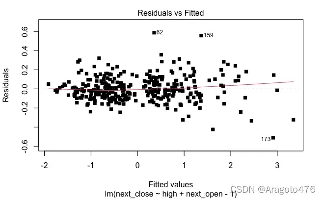
图8 残差直方图图9 残差与预测值散点图

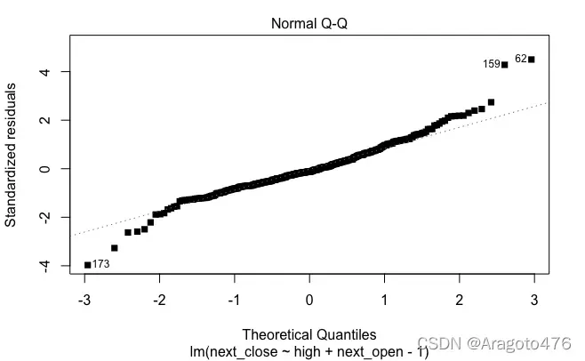
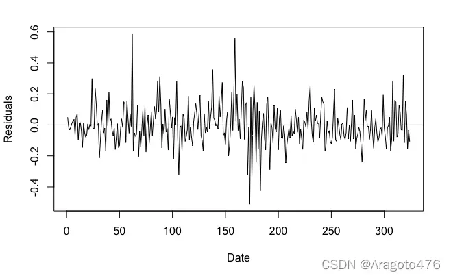
图10 QQ图图11 残差时序图

上面的残差图表明该模型具有轻微的异方差性，并且残差可能是自相关的。

4.多重共线性

(1) 诊断

1. 相关系数

library(corrplot)

corrplot.mixed(cor(train.scale[,-8]), lower = "ellipse", upper = "circle", addCoef.col="royalblue4", addCoefasPercent=T, tl.col="black", tl.cex=0.5)

输出：

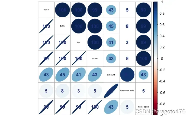
图13 相关系数图

上图显示开盘价、最高价、最低价、收盘价与次日开盘价存在严重共线性；周转率与周转率存在严重的共线性。

2. 方差膨胀因子(VIF)

vif(sol.lm1)

输出：

         open          high           low         close        amount 
     275.4309      408.0849      453.7918      454.8052       58.8605 
turnover_rate     next_open 
      45.1622      161.2500

结果表明模型存在严重的多重共线性。

3. 特征系统分析

train.cor = cor(train.scale[,-8])

ev <- eigen(train.cor)
ev$values  # 特征值

kappa(train.cor, exact = T) # kappa系数

输出：

[1] 5.224278607 1.743623915 0.015066957 0.010401233 0.003231141
[6] 0.002356826 0.001041320

[1] 5016.979

Kappa系数为5016.979。结果显示模型中存在多重共线性。

(2) 主成分回归

1. 主成分分析

train.pca1 = princomp(~open+high+low+close+amount+turnover_rate+next_open, data = train.scale, cor=T)
screeplot(train.pca1, type="l", main="", lwd=2, pch=15) #碎石图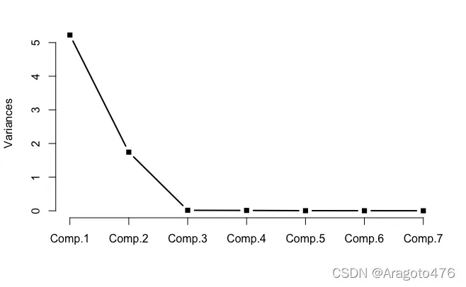

图14 碎石图

summary(train.pca1, loadings=T)

输出：

Importance of components:
                          Comp.1    Comp.2      Comp.3     Comp.4
Standard deviation     2.2856681 1.3204635 0.122747533 0.10198644
Proportion of Variance 0.7463255 0.2490891 0.002152422 0.00148589
Cumulative Proportion  0.7463255 0.9954146 0.997567068 0.99905296
                             Comp.5       Comp.6       Comp.7
Standard deviation     0.0568431282 0.0485471564 0.0322694827
Proportion of Variance 0.0004615916 0.0003366895 0.0001487599
Cumulative Proportion  0.9995145506 0.9998512401 1.0000000000

Loadings:
              Comp.1 Comp.2 Comp.3 Comp.4 Comp.5 Comp.6 Comp.7
open           0.433         0.583  0.325  0.329  0.240  0.439
high           0.435                      -0.532  0.565 -0.438
low            0.432  0.113  0.106  0.287        -0.651 -0.523
close          0.433        -0.323        -0.501 -0.321  0.582
amount         0.238 -0.633  0.326 -0.638        -0.165       
turnover_rate        -0.743 -0.297  0.581         0.120       
next_open      0.432        -0.584 -0.245  0.587  0.234

从碎石图中，我们发现前两个主成分就已经可以解释大部分方差来源（99.54%），因此选择前两个主成分进行后续分析。成分矩阵如下所示：

	主成分1	主成分2
x1	0.4325	0.0952
x2	0.4347	0.0781
x3	0.4321	0.1127
x4	0.4332	0.0981
x5	0.2379	-0.6329
x6	0.0783	-0.7432
x7	0.4323	0.0982

由于主成分1中，价格因素（开盘价、收盘价、最高最低价）系数绝对值较大；而主成分2中数量因素（成交额、换手率）系数绝对值较大，因此可以将主成分1解释为价格因子，将主成分2解释为数量因子。改进后的模型为：

$y=\alpha_1\ F_1+\alpha_2\ F_2+\varepsilon$

train.score = train.pca1$scores[,1:2]

train.z1 = train.score[,1]
train.z2 = train.score[,2]
train.pca.data = data.frame(train.scale$next_close, train.z1, train.z2)

names(train.pca.data) = c("next_close", "z1", "z2")

train.pcr = lm(next_close ~ .-1, data = train.pca.data)

summary(train.pcr)

输出：

Call:
lm(formula = next_close ~ . - 1, data = train.pca.data)

Residuals:
     Min       1Q   Median       3Q      Max 
-0.51908 -0.09033 -0.01348  0.07358  0.64094 

Coefficients:
   Estimate Std. Error t value Pr(>|t|)    
z1 0.428311   0.003609  118.67   <2e-16 ***
z2 0.097589   0.006247   15.62   <2e-16 ***
---
Signif. codes:  0 ‘***’ 0.001 ‘**’ 0.01 ‘*’ 0.05 ‘.’ 0.1 ‘ ’ 1

Residual standard error: 0.1485 on 322 degrees of freedom
Multiple R-squared:  0.978,	Adjusted R-squared:  0.9779 
F-statistic:  7164 on 2 and 322 DF,  p-value: < 2.2e-16

回归系数的最小二乘估计分别为0.4283和0.0976。

2. 主成分回归

# 标准化变量的系数
xs.s = c(train.pca1$loadings[,1] * train.pcr$coefficients[1] + train.pca1$loadings[,2] * train.pcr$coefficients[2])

# 原变量的系数
xs.o = xs.s
for (i in 1:length(xs.s)){
  xs.o[i+1] = xs.s[i] * sd(train.data$next_close) / sd(train.data[, i])
}
xs.o[1] = mean(train.data$next_close) - sum(xs.o[2:8] * apply(train.data[,-8], 2, mean))

上述结果表示为原始标准化回归变量，如下：

$y\widehat\\^\ast\ =0.1945x_1^\ast+0.1938x_2^\ast+0.1961x_3^\ast+0.1951x_4^\ast+0.0401x_5^\ast-0.0390x_6^\ast+0.1947x_7^\ast$

对于非标准化回归量，有：

$y\widehat\\ =2.7641+0.1903x_1+0.1871x_2+0.2014x_3+0.1940x_4+0.0000006x_5-2.0772x_6+0.1916x_7$

(3) 岭回归

library(MASS)
train.ridge = lm.ridge(next_close ~ ., train.scale, scale = F, center = F, lambda=seq(0,7, length.out=1000), y=T, x=T)
beta = coef(train.ridge)

la = train.ridge$lambda[which.min(train.ridge$GCV)]
coe = train.ridge$coef[,which.min(train.ridge$GCV)]

matplot(train.ridge$lambda,t(train.ridge$coef),xlab = expression(lambda),ylab = "Coefficients",type = "l",lty = 1:7, col=1:7)
legend("topright", inset=0.05,legend=names(train.data)[-8],cex=0.8,col=1:7,lty=1:7, nc=3)
abline(v=train.ridge$lambda[which.min(train.ridge$GCV)], col="gray", lty=2, lwd=2)
text("Smallest GDV", x=1, y=0.4, col="gray")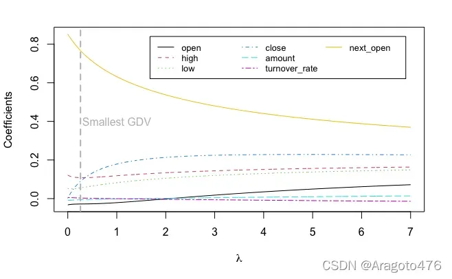

图15 岭迹图

coe # 标准化

coe.o = rep(0, 8)
for (i in 1:length(coe)){
  coe.o[i+1] = coe[i] * sd(train.data$next_close) / sd(train.data[, i])
}
coe.o[1] = mean(train.data$next_close) - sum(coe.o[2:8] * apply(train.data[,-8], 2, mean))
coe.o # 原始

对于标准化回归变量，经验回归方程为：

$y\widehat\\^\ast\ =-0.0279x_1^\ast+0.1083x_2^\ast+0.0557x_3^\ast+0.0896x_4^\ast-0.0058x_5^\ast+0.0031x_6^\ast+0.7668x_7^\ast$

对于原始回归变量，经验回归方程为：

$y\widehat\\ =1.6529-0.0273x_1+0.1046x_2+0.0572x_3+0.0891x_4-0.00000008x_5-0.1669x_6+0.7544x_7$

五、模型效果及结果分析

(1) 训练集

# 变量选择的模型
p1.1 = predict(sol.lm3, train.data) # 预测价格
r1.1 = p1.1 - train.data$next_close # 偏差率

# 主成分回归的模型
p2.1 = cbind(1, as.matrix(train.data[,-8])) %*% xs.o # 预测价格
r2.1 = p2.1 - train.data$next_close # 偏差率

# 岭回归的模型
p3.1 = cbind(1, as.matrix(train.data[, -8])) %*% coe.o # 预测价格
r3.1 = p3.1 - train.data$next_close # 偏差率

# 预测价格可视化
train.PRE = data.frame("VS"=p1.1, "PCR"=p2.1, "RR"=p3.1, "Org"=train.data$next_close)

g1 = ggplot(train.PRE, aes(x=1:324))
# 变量选择的模型
g1 + geom_line(aes(y=VS,colour=I("orange2")), lwd=1) + 
  geom_line(aes(y=Org, colour=I("darkblue")), lwd=1) + 
  labs(x="Trade Date",y = "Close Price(RMB)") + 
  scale_color_manual(name = "", values=c("darkblue", "orange2"),labels=c("Original", "Variable Selection")) + 
    theme_economist() + theme(legend.position = "top")

# 主成分回归的模型
g1 + geom_line(aes(y=PCR,colour=I("red3")), lwd=1) + 
  geom_line(aes(y=Org, colour=I("darkblue")), lwd=1) + 
  labs(x="Trade Date",y = "Close Price(RMB)") + 
  scale_color_manual(name = "", values=c("darkblue", "red3"),labels=c("Original", "PCR")) + 
    theme_economist() + theme(legend.position = "top")

# 岭回归的模型
g1 + geom_line(aes(y=RR,colour=I("green3")), lwd=1) + 
  geom_line(aes(y=Org, colour=I("darkblue")), lwd=1) + 
  labs(x="Trade Date",y = "Close Price(RMB)") + 
  scale_color_manual(name = "Method", values=c("darkblue", "green3"),labels=c("Original", "RR")) + 
    theme_economist() + theme(legend.position = "top")

# 偏差率可视化
train.ER = data.frame("VS"=r1.1, "PCR"=r2.1, "RR"=r3.1)/train.data$next_close

# 分布
ggplot(train.ER) + geom_density(aes(x=VS,colour=I("orange2")), lwd=1)+
  geom_density(aes(x=PCR,colour=I("red3")), lwd=1) +
  geom_density(aes(x=RR,colour=I("green3")), lwd=1) +
  labs(x="Error Rate",y = "Density") + 
  scale_color_manual(name = "Method", values=c("green3", "orange2", "red3"),labels=c("RR", "VS", "PCR"))

# 箱线图
ggplot(train.ER)+geom_boxplot(aes(x=factor("VS"),y=VS, fill = I("orange2")))+geom_boxplot(aes(x=factor("PCR"),y=PCR, fill = I("red3")))+geom_boxplot(aes(x=factor("RR"),y=RR, fill = I("green3")))+
  labs(x="Method",y = "Error Rate")

输出：

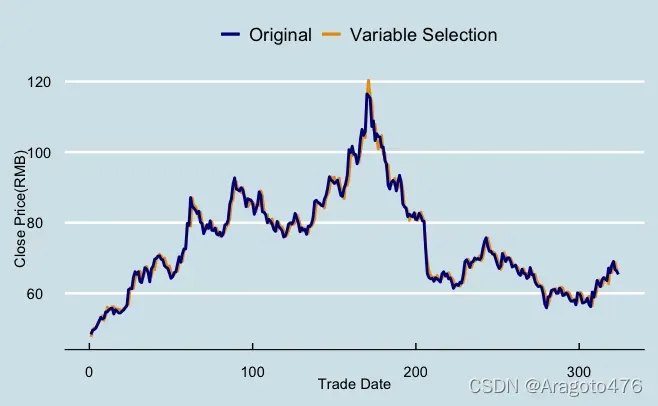
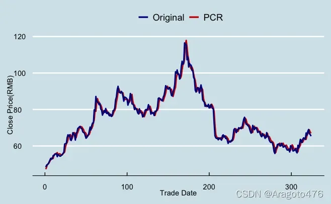
图16 变量选择拟合效果图17 主成分回归拟合效果

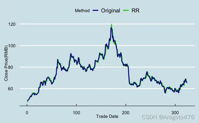
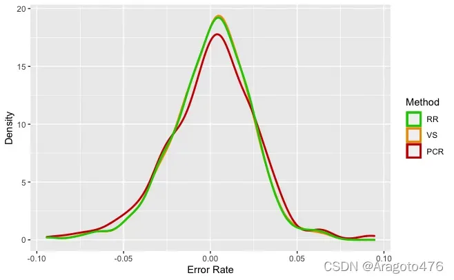
图18 岭回归拟合效果图19 不同方法偏差率的分布

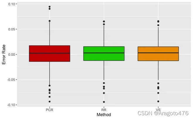
图20 不同方法偏差率的箱线图

以上图片可以看到，三种方法在训练集上的拟合效果基本一致，且效果不错，具体而言：变量选择、主成分回归以及岭回归的平均预测偏差率分别为0.0589%、0.0739%、0.0639%；1/4及3/4分位数的绝对值均小于1.8%；中位数分别为0.3093%、0.2409%、0.2856%。

(2) 测试集

# 变量选择的模型
p1.2 = predict(sol.lm3, test.data) # 预测价格
r1.2 = p1.2 - test.data$next_close # 偏差率

# 主成分回归的模型
p2.2 = cbind(1, as.matrix(test.data[,-8])) %*% xs.o # 预测价格
r2.2 = p2.2 - test.data$next_close # 偏差率

# 岭回归的模型
p3.2 = cbind(1, as.matrix(test.data[, -8])) %*% coe.o # 预测价格
r3.2 = p3.2 - test.data$next_close # 偏差率

# 预测价格可视化
test.PRE = data.frame("VS"=p1.2, "PCR"=p2.2, "RR"=p3.2, "Org"=test.data$next_close)

g2 = ggplot(test.PRE, aes(x=1:50))

# 变量选择的模型
g2 + geom_line(aes(y=VS,colour=I("orange2")), lwd=1) + 
  geom_line(aes(y=Org, colour=I("darkblue")), lwd=1) + 
  labs(x="Trade Date",y = "Close Price(RMB)") + 
  scale_color_manual(name = "", values=c("darkblue", "orange2"),labels=c("Original", "Variable Selection")) + 
    theme_economist() + theme(legend.position = "top")

# 主成分回归的模型  
g2 + geom_line(aes(y=PCR,colour=I("red3")), lwd=1) + 
  geom_line(aes(y=Org, colour=I("darkblue")), lwd=1) + 
  labs(x="Trade Date",y = "Close Price(RMB)") + 
  scale_color_manual(name = "", values=c("darkblue", "red3"),labels=c("Original", "PCR")) + 
    theme_economist() + theme(legend.position = "top")

# 岭回归的模型
g2 + geom_line(aes(y=RR,colour=I("green3")), lwd=1) + 
  geom_line(aes(y=Org, colour=I("darkblue")), lwd=1) + 
  labs(x="Trade Date",y = "Close Price(RMB)") + 
  scale_color_manual(name = "Method", values=c("darkblue", "green3"),labels=c("Original", "RR")) + 
    theme_economist() + theme(legend.position = "top")

# 偏差率可视化
test.ER = data.frame("VS"=r1.2, "PCR"=r2.2, "RR"=r3.2)/test.data$next_close

# 分布
ggplot(test.ER) + geom_density(aes(x=VS,colour=I("orange2")), lwd=1)+
  geom_density(aes(x=PCR,colour=I("red3")), lwd=1) +
  geom_density(aes(x=RR,colour=I("green3")), lwd=1) +
  labs(x="Error Rate",y = "Density") + 
  scale_color_manual(name = "Method", values=c("green3", "orange2", "red3"),labels=c("RR", "VS", "PCR"))

# 箱线图
ggplot(test.ER)+geom_boxplot(aes(x=factor("VS"),y=VS, fill = I("orange2")))+geom_boxplot(aes(x=factor("PCR"),y=PCR, fill = I("red3")))+geom_boxplot(aes(x=factor("RR"),y=RR, fill = I("green3")))+
  labs(x="Method",y = "Error Rate")

输出：

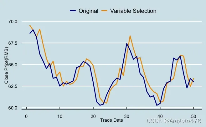
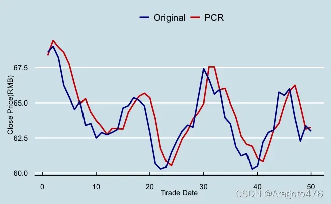
图21 变量选择预测效果图22 主成分回归预测效果

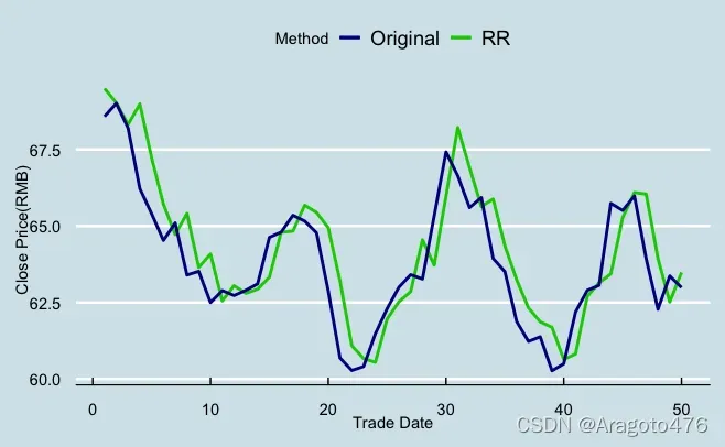
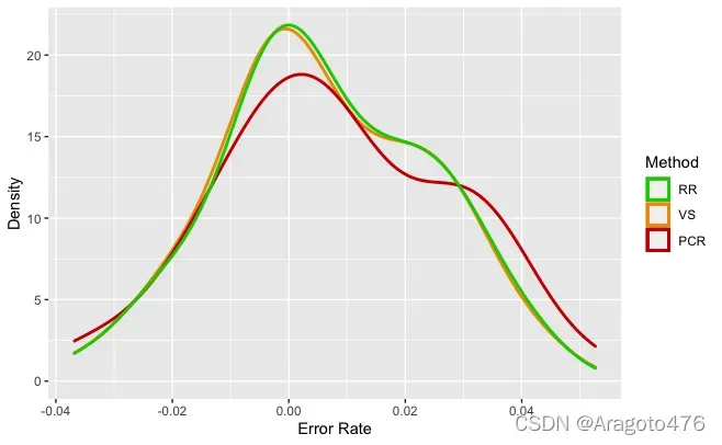
图23 岭回归预测效果图24 不同方法偏差率的分布

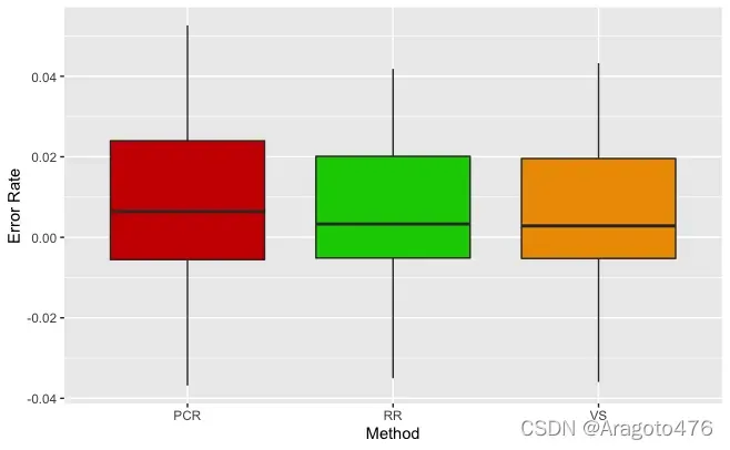
图25 不同方法偏差率的箱线图

以上图片可以看到，变量选择及岭回归在测试集上的预测效果基本一致，而主成分回归的预测效果稍显逊色。具体而言：变量选择、主成分回归以及岭回归的平均预测偏差率分别为0.6086%、0.7924%、0.6430%；1/4及3/4分位数的绝对值均小于2.4%；中位数分别为0.2837%、0.6406%、0.3295%。

原文链接：https://blog.csdn.net/weixin_60975498/article/details/123163289

运用R语言、Tushare对单支股票进行回归分析

一、数据说明

(1) 数据的获取

(2) 数据预处理与分析

2.初步回归分析

(1) 模型和变量

(2) 参数估计

(3) 假设检验

1. 回归显著性检验

2. 回归系数的显著性检验

3. 回归子集的显著性检验

3.变量选择

(1) 最优子集选择

(2) 逐步回归

(3) 最终模型

(4) 假设检验

1. 回归显著性检验

2. 回归系数的显著性检验

(6) 残差分析

4.多重共线性

(1) 诊断

1. 相关系数

2. 方差膨胀因子(VIF)

3. 特征系统分析

(2) 主成分回归

1. 主成分分析

2. 主成分回归

(3) 岭回归

五、模型效果及结果分析

(1) 训练集

(2) 测试集

相关推荐