1、rvctools下载安装
rvctools下载地址:rvctools下载
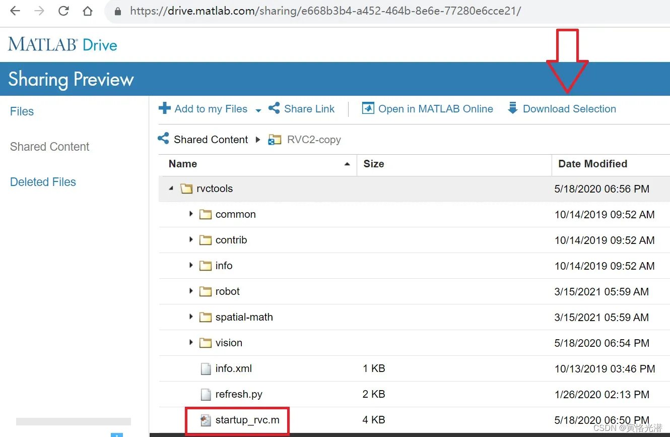
截图如下,点击红色箭头指示的“Download Shared Folder” 即可下载
下载之后进行解压,解压到D:\MATLAB\toolbox这个工具箱目录,这个安装路径根据自己的情况来选择,没有安装MATLAB,感兴趣的可以查阅:MatLab的下载、安装与使用(亲测有效)
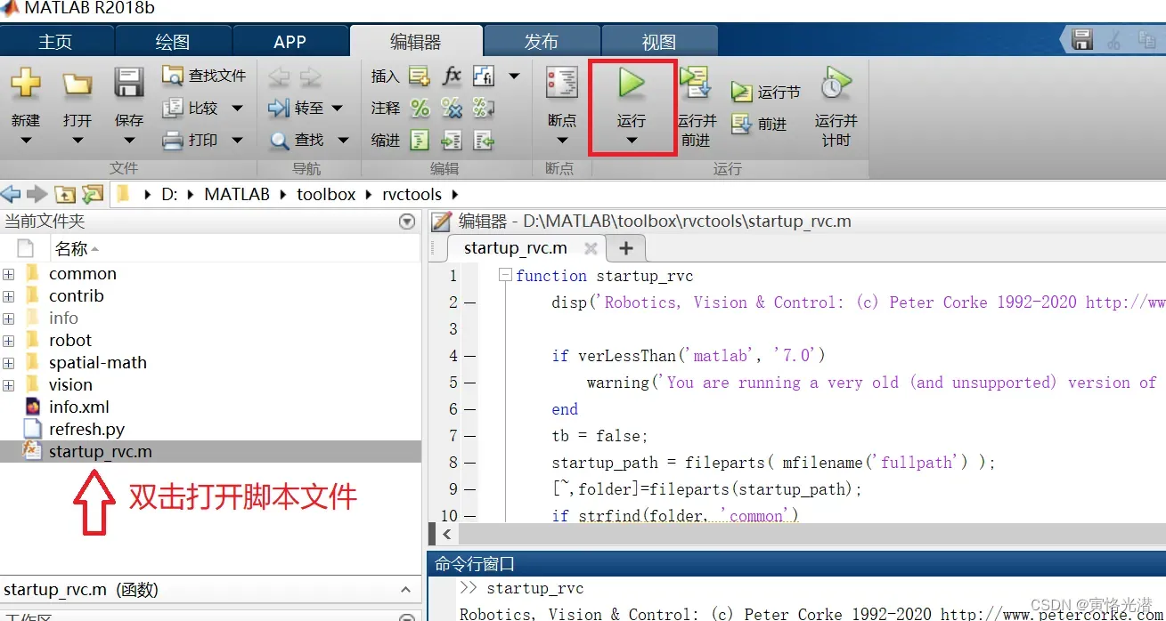
然后我们打开MATLAB,打开上面解压的这个机器人工具箱,双击startup_rvc.m,点击运行,如下图:
这样就愉快的安装好了这个机器人工具箱了,其中startup_rvc.m的代码如下:
function startup_rvc
    disp('Robotics, Vision & Control: (c) Peter Corke 1992-2020 http://www.petercorke.com')

    if verLessThan('matlab', '7.0')
        warning('You are running a very old (and unsupported) version of MATLAB.  You will very likely encounter significant problems using the toolboxes but you are on your own with this');
    end
    tb = false;
    startup_path = fileparts( mfilename('fullpath') );
    [~,folder]=fileparts(startup_path);
    if strfind(folder, 'common')
        % startup_rvc is in common folder
        rvcpath = fileparts(startup_path);
    else
        % startup_rvc is in folder above common
        rvcpath = startup_path;
    end

    robotpath = fullfile(rvcpath, 'robot');
    if exist(robotpath, 'dir')
        addpath(robotpath);
        tb = true;
        if exist('startup_rtb') == 2
            startup_rtb
        end
    end

    visionpath = fullfile(rvcpath, 'vision');
    if exist(visionpath, 'dir')
        addpath(visionpath);
        tb = true;
        if exist('startup_mvtb') == 2
            startup_mvtb
        end
    end

    if tb
        % RTB or MVTB is present

        % add spatial math toolbox
        p = fullfile(rvcpath, 'spatial-math');
        if exist(p, 'dir')
            try
                fp = fopen( fullfile(p, 'RELEASE'), 'r');
                release = fgetl(fp);
                fclose(fp);
            catch ME
                release = [];
            end
            if release
                release = ['(release ' release ')'];
            else
                release = '';
            end
            fprintf('- Spatial Math Toolbox for MATLAB %s\n', release)
            addpath(p);
        end

        % add common files
        addpath(fullfile(rvcpath, 'common'));
    else
        fprintf('Neither Robotics Toolbox or MachineVision Toolbox found in %s\n', rvcpath);
    end

    % check for any install problems
    rvccheck(false)
end后期如果关闭了MATLAB,想要运行机器人的话,运行函数startup_rvc即可
2、运动学
机器人或者说飞行器,随着时间而发生动作变换,叫做运动学(kinematics),这个跟动力学(dynamics)是不一样的,动力学是研究影响运动的因素,而动力学是不考虑作用力和质量等因素,研究的是随着时间在空间中的位置问题。对于运动基本上就是平移和旋转了,就会牵涉到坐标系和角度等转换,接下来我们来学习下
2.1、平移
物体的平移比较简单,就是沿着XYZ三轴平移
沿着X轴平移:transl(2,0,0)
沿着Y轴平移:transl(0,2,0)
沿着Z轴平移:transl(0,0,2)
当然也可以在XYZ轴都进行平移:transl(1,3,2)
我们对最后这个画图看下效果:trplot(transl(1,3,2)),如下图:
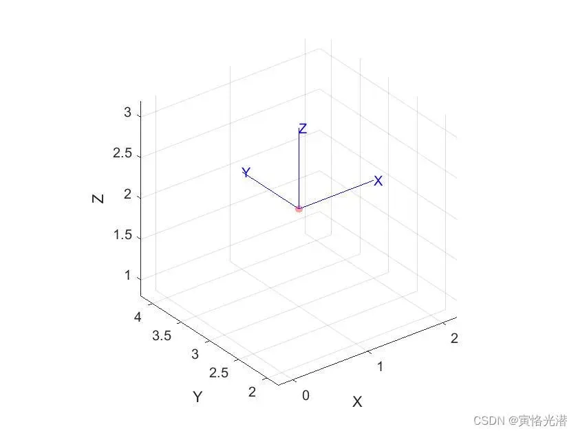
我标注红点的位置是(1,3,2),因为是在三维空间的展示,所以看起来XYZ轴的数值不对,其实是对的,大家可以在MATLAB中的这张图进行拖动旋转,然后就会发现红点的坐标就是(1,3,2)
2.2、旋转
旋转就是绕轴做圆周运动
绕X轴旋转:Rx = rotx(pi/2)
绕Y轴旋转:Ry = roty(pi/2)
绕Z轴旋转:Rz = rotz(pi/2)
旋转叠加:Rxy = Rx * Ry
动画演示:tranimate(Rxy),这样看起来非常清晰直观。
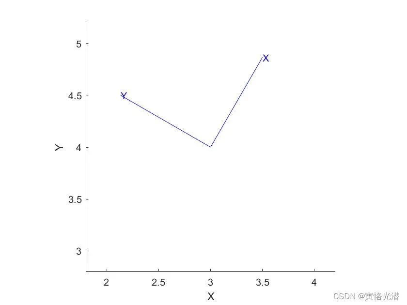
我们来看下点(3,4),旋转60度的情况:
T1=SE2(3,4,pi/3)

T1 =
    0.5000   -0.8660         3
    0.8660    0.5000         4
         0         0         1
对其画图:trplot(T1),如下:
我们也可以使用transforms3d库中的结果,用来验证在MATLAB中生成的结果,代码如下:
import transforms3d as tfs
import math
print(tfs.euler.euler2mat(math.pi/3,0,0))
/*
[[ 1.         0.         0.       ]
 [ 0.         0.5       -0.8660254]
 [-0.         0.8660254  0.5      ]]
*/
MATLAB中的结果如下:
T2=rotx(pi/3)
/*
T2 =

    1.0000         0         0
         0    0.5000   -0.8660
         0    0.8660    0.5000
*/
上述是弧度制,也可以使用角度制, 指定deg参数:rotx(60,’deg’)
3、六轴机器人
3.1、Link关节连杆
这里我们使用更改的D-H参数,也就是接下来的Link函数指定modified参数
L = Link([1 2 3 4],'modified')
%L = Revolute(mod): theta=q, d=2, a=3, alpha=4, offset=0Link函数里面的参数分别表示为,关节角度[L1.theta]、连杆偏距[L1.d]、连杆长度[L1.a]、连杆旋转角度[L1.alpha],参数modified表示的是改进版本的DH参数
这里附带介绍下D-H的相关知识:
DH参数是一种描述机器人关节之间关系的参数化方法,由Denavit和Hartenberg提出。DH参数法可以用4个参数来表示刚体之间的相对关系,包括沿Z轴的平移长度a、沿共同法线的旋转角度α、在XZ平面内的偏移距离d、绕Z轴的旋转角度θ。
DH参数在ROS中被广泛应用,用于描述机器人关节和坐标系之间的关系,主要用于正向运动学计算,可以通过DH表获取每个关节的变换矩阵,将所有变换矩阵相乘,最终获得从基准坐标系到末端执行器坐标系的变换矩阵。
这个D-H方法是在运动学中求解比较通用的,其余还有李代数方法等。
连杆类型
L.type()
%ans = 'R'也就是说这个是旋转的R(revolute)关节类型,除此之外还有一种是柱状形(prismatic)的关节
接下来就是分别创建6个关节,也就是为6轴的机械臂做准备:
L1 = Link([0 0 0 0],'modified')
L2 = Link([0 0.138+0.024 0 -pi/2],'modified')
L3 = Link([0 -0.127-0.024 0.42 0],'modified')
L4 = Link([0 0.114+0.021 0.375 0],'modified')
L5 = Link([0 0.114+0.021  0 -pi/2],'modified')
L6 = Link([0 0.09+0.021  0 pi/2],'modified')
3.2、SerialLink机械臂
上面定义好了6个关节,接下来我们使用SerialLink将这些关节连接起来成为一个六轴机械臂的机器人。
MyBot = SerialLink([L1,L2,L3,L4,L5,L6],'name','Six Axis Robot')我们先来看下SerialLink有哪些方法:help(SerialLink)
— SerialLink 的帮助 —
SerialLink Serial-link robot class
A concrete class that represents a serial-link arm-type robot. Each link
and joint in the chain is described by a Link-class object using Denavit-Hartenberg
parameters (standard or modified).
Constructor methods::
SerialLink general constructor
L1+L2 construct from Link objects
Display/plot methods::
animate animate robot model
display print the link parameters in human readable form
dyn display link dynamic parameters
edit display and edit kinematic and dynamic parameters
getpos get position of graphical robot
plot display graphical representation of robot
plot3d display 3D graphical model of robot
teach drive the graphical robot
Testing methods::
islimit test if robot at joint limit
isconfig test robot joint configuration
issym test if robot has symbolic parameters
isprismatic index of prismatic joints
isrevolute index of revolute joints
isspherical test if robot has spherical wrist
isdh test if robot has standard DH model
ismdh test if robot has modified DH model
Conversion methods::
char convert to string
sym convert to symbolic parameters
todegrees convert joint angles to degrees
toradians convert joint angles to radians
从SerialLink类提供的方法,我们了解到可以用来描述机器人的连杆结构:SerialLink类描述机器人的连杆结构,包括每个连杆的长度、方向和旋转轴。有了这些信息,我们可以用于计算机器人的运动学模型,从而对机器人做出控制和运动规划。
显示连接参数:MyBot.display()
MyBot =

Six Axis Robot:: 6 axis, RRRRRR, modDH, slowRNE
+---+-----------+-----------+-----------+-----------+-----------+
| j |     theta |         d |         a |     alpha |    offset |
+---+-----------+-----------+-----------+-----------+-----------+
|  1|         q1|          0|          0|          0|          0|
|  2|         q2|      0.162|          0|    -1.5708|          0|
|  3|         q3|     -0.151|       0.42|          0|          0|
|  4|         q4|      0.135|      0.375|          0|          0|
|  5|         q5|      0.135|          0|    -1.5708|          0|
|  6|         q6|      0.111|          0|     1.5708|          0|
+---+-----------+-----------+-----------+-----------+-----------+操作机械臂:MyBot.teach()
这样就会生成六轴机械臂的机器人,然后我们就可以通过操作不同关节来操作机器人的机械臂了,如下图:
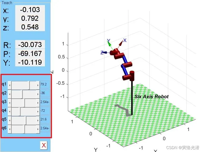
我们操作左边q1~q6,就会看到机械臂的运动以及XYZ轴和RPY欧拉角的变化
4、运动学
4.1、正运动学
运动学分为正解和逆解,正运动学(Forward kinematics):已知每个关节的位姿与连杆的长度等参数,求解末端执行器的位姿。
我们来看下正解
MyBot.fkine([pi/2 -pi/4 pi/2 pi/3 -pi/2 pi/6])
/*
ans =
   -0.8660    0.5000         0    -0.146
   -0.4830   -0.8365    0.2588    0.4605
    0.1294    0.2241    0.9659     0.174
         0         0         0         1
*/
生成的是对应关节角度的末端的齐次变换矩阵。
4.2、逆运动学
逆运动学(Inverse kinematics)跟正运动学是反过来的,根据机器人的末端执行器的位姿,计算出机器人各个关节的位姿等运动参数。这个要复杂点,因为它的求解可能是不确定的唯一解,会产生多重解的问题,当然也可能得不到解析解的情况。
迭代法:
%起始状态
init = [0.795 0.257 -0.135 0 0 -pi/2]
%目标状态
targ = [0 0.836 -0.135 0 -pi/3 -pi/2]
T0=MyBot.fkine(init)
/*
T0 =
    0.0852    0.6951   -0.7139    0.3501
    0.0869    0.7086    0.7003    0.7239
    0.9926   -0.1217         0   -0.2864
         0         0         0         1
*/
TF=MyBot.fkine(targ)
/*
TF =
    0.6450    0.3821   -0.6618    0.4076
         0    0.8660    0.5000    0.2015
    0.7642   -0.3225    0.5586   -0.5947
         0         0         0         1
*/
%每次迭代的末端执行器相对于首端的齐次变换矩阵
step =50
%ctraj是Matlab中机器人轨迹(trajectory)规划的函数
TC=ctraj(T0,TF,step)
%比如迭代到第50次
/*
TC(50) =
    0.6450    0.3821   -0.6618    0.4076
         0    0.8660    0.5000    0.2015
    0.7642   -0.3225    0.5586   -0.5947
         0         0         0         1
*/
qq = MyBot.ikine(TC,'mask',[1 1 1 0 0 0])返回的就是50*6的双精度数组,长度是50:length(qq)
0.7951 0.1852 0.0167 -0.0314 0.0432 0
0.7946 0.1853 0.0174 -0.0303 0.0422 0
0.7931 0.1856 0.0196 -0.0267 0.0394 0
……
-0.1278 0.6478 0.4212 0.2245 -0.2429 0
-0.1317 0.6494 0.4203 0.2230 -0.2419 0
-0.1330 0.6500 0.4201 0.2226 -0.2416 0
接下来我们使用ctraj来规划轨迹,使用ikine函数来做逆解,沿着轨迹进行运动。
5、直线轨迹规划
这里使用标准的DH参数来测试下,三个自由度的机械臂如何做运动规划的,一起来了解下:
%这里是第一次开启MATLAB时,运行这个函数,启动rvc:startup_rvc
%参数:关节角、偏置距离、连杆长度、连杆扭角、sigma为0表示旋转关节
L1 = Link([0 84.72 41.04 pi/2 0]);
L2 = Link([0 0 200 0 0]);
L3 = Link([0 0 214.8 0 0]);
% 可以限制旋转角度范围
L1.qlim = [deg2rad(-170) deg2rad(170)];
L2.qlim = [deg2rad(-60) deg2rad(85)];
L3.qlim = [deg2rad(-90) deg2rad(10)];
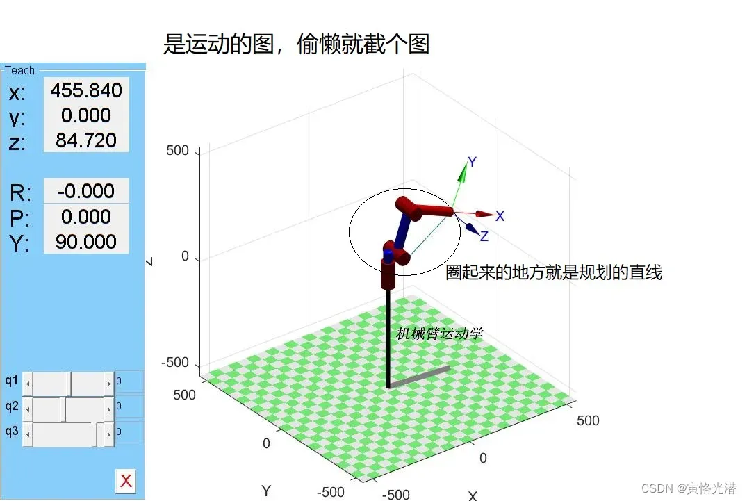
Bot2 = SerialLink([L1 L2 L3], 'name', '机械臂运动学');
%手动操作关节进行旋转
Bot2.teach()
%起点
T1 = transl(100,-10,50);
%终点
T2 = transl(300,-30,200);
%规划轨迹(trajectory)
T = ctraj(T1,T2,50);
Tj = transl(T);
%输出末端轨迹
plot3(Tj(:,1),Tj(:,2),Tj(:,3));
%当反解的机械臂自由度少于6时,要用mask掩码减少自由度,否则无法直接调用ikine作为运动学反解函数
q = Bot2.ikine(T,'mask',[1 1 1 0 0 0]);
Bot2.plot(q);
这样就会看到沿着规划好的直线,自动进行运动了,简单起见截个图如下(实质是运动的):
6、圆轨迹规划
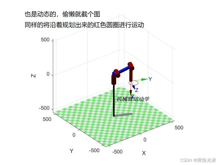
N = (0:0.5:100)';
center = [200 -150 -50];
radius = 60;
theta = (N/N(end))*2*pi;
points = (center + radius*[cos(theta) sin(theta) zeros(size(theta))])';
plot3(points(1,:),points(2,:),points(3,:),'r');

%沿着圆的轨迹平移
T = transl(points');
q2 = Bot2.ikine(T,'mask',[1 1 1 0 0 0]);
Bot2.plot(q2);
这样就会看到沿着规划好的圆,自动进行运动了,简单起见截个图如下(实质是运动的):
7、常见用法
其余的一些常见用法,如下:
关节数:MyBot.n
画出机械臂:MyBot.plot([0 0 0 0 0 0])
机器人的结构类型:Mybot.config
关节范围:MyBot.qlim
连杆向量(更直观):MyBot.links
重力方向([gx gy gz]):MyBot.gravity
连杆的动力学属性:MyBot.dyn
是否是旋转关节:MyBot.isrevolute
是否是移动关节:MyBot.isprismatic
是否是球关节:MyBot.isspherical
关节与连杆是否有符号参数:MyBot.issym
可以编辑动力学参数:MyBot.edit
8、小结
文章主要介绍了机器人工具箱rvctools,以及它的用法,了解运动学的相关知识,对坐标的变换,轨迹的规划等有个直观的了解,最后在进行运动规划的时候,有时候会出现下面这样的错误:
警告: failed to converge: try a different initial value of joint coordinates
收敛失败:尝试不同的关节坐标初始值
这样的情况一般是关节不能到达那个坐标,所以需要更改坐标为合理值即可。
另外仔细观察代码中会出现一些矩阵带单引号‘,这个表示转置的意思,比如:
size(N)的形状是1 x 201,而size(N’)的形状就是201 x 1
元素个数numel(N) 结果:201,维度ndims(N) 结果:2
文章出处登录后可见!