机器学习与深度学习——通过决策树算法分类鸢尾花数据集iris求出错误率画出决策树并进行可视化

什么是决策树？

决策树是一种常用的机器学习算法，它可以对数据集进行分类或回归分析。决策树的结构类似于一棵树，由节点和边组成。每个节点代表一个特征或属性，每个边代表一个判断或决策。从根节点开始，根据特征的不同取值，不断向下遍历决策树，直到达到叶子节点，即最终的分类或回归结果。

在分类问题中，决策树通过将数据集分成不同的类别来进行分类。在回归问题中，决策树通过将数据集分成不同的区域来进行回归分析。

决策树的优点包括易于理解和解释、能够处理具有非线性关系的数据、对缺失数据具有容忍性等。然而，决策树也存在一些缺点，例如容易过拟合、对噪声数据敏感等。为了解决这些问题，常常需要对决策树进行剪枝或使用集成学习算法如随机森林来提高预测准确性。

两个目标

1、通过决策树算法对iris数据集前两个维度的数据进行模型训练并求出错误率，最后进行可视化展示数据区域划分。
2、通过决策树算法对iris数据集总共四个维度的数据进行模型训练并求出错误率。

基本思路：

1、先载入iris数据集 Load Iris data
2、分离训练集和设置测试集split train and test sets
3、使用决策树模型进行训练Train using clf
4、画出决策树
5、然后二维进行可视化处理Visualization
6、最后通过绘图决策平面plot decision plane

程序代码

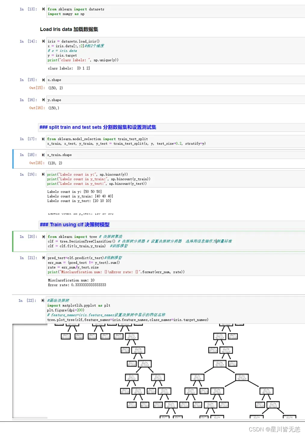
1、通过决策树算法对iris数据集前两个维度的数据进行模型训练并求出错误率，最后进行可视化展示数据区域划分：

from sklearn import datasets
import numpy as np
### Load Iris data 加载数据集
iris = datasets.load_iris()
x = iris.data[:,:2]#前2个维度
# x = iris.data
y = iris.target
print("class labels: ", np.unique(y))
x.shape
y.shape

### split train and test sets
from sklearn.model_selection import train_test_split
x_train, x_test, y_train, y_test = train_test_split(x, y, test_size=0.2, stratify=y)
x_train.shape
print("Labels count in y:", np.bincount(y))
print("Labels count in y_train:", np.bincount(y_train))
print("Labels count in y_test:", np.bincount(y_test))

### Train using clf 决策树模型
from sklearn import tree # 决策树算法
clf = tree.DecisionTreeClassifier() # 决策树分类器 # 设置决策树分类器  选择用信息熵作为测量标准
clf = clf.fit(x_train,y_train)  #训练模型
pred_test=clf.predict(x_test)#预测模型
err_num = (pred_test != y_test).sum()
rate = err_num/y_test.size
print("Misclassfication num: {}\nError rate: {}".format(err_num, rate))#计算错误率

#画出决策树
import matplotlib.pyplot as plt
plt.figure(dpi=200)
# feature_names=iris.feature_names设置决策树中显示的特征名称
tree.plot_tree(clf,feature_names=iris.feature_names,class_names=iris.target_names)

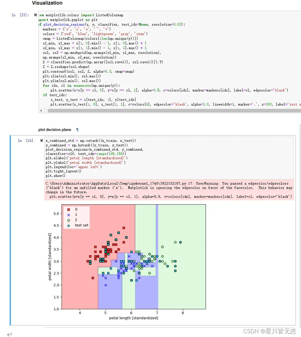
### Visualization
from matplotlib.colors import ListedColormap
import matplotlib.pyplot as plt
def plot_decision_regions(x, y, classifier, test_idx=None, resolution=0.02):
    markers = ('s', 'x', 'o', '^', 'v')
    colors = ('red', 'blue', 'lightgreen', 'gray', 'cyan')
    cmap = ListedColormap(colors[:len(np.unique(y))])
    x1_min, x1_max = x[:, 0].min() - 1, x[:, 0].max() + 1
    x2_min, x2_max = x[:, 1].min() - 1, x[:, 1].max() + 1
    xx1, xx2 = np.meshgrid(np.arange(x1_min, x1_max, resolution),
    np.arange(x2_min, x2_max, resolution))
    Z = classifier.predict(np.array([xx1.ravel(), xx2.ravel()]).T)
    Z = Z.reshape(xx1.shape)
    plt.contourf(xx1, xx2, Z, alpha=0.3, cmap=cmap)
    plt.xlim(xx1.min(), xx1.max())
    plt.ylim(xx2.min(), xx2.max())
    for idx, cl in enumerate(np.unique(y)):
        plt.scatter(x=x[y == cl, 0], y=x[y == cl, 1], alpha=0.8, c=colors[idx], marker=markers[idx], label=cl, edgecolor='black')
    if test_idx:
        x_test, y_test = x[test_idx, :], y[test_idx]
        plt.scatter(x_test[:, 0], x_test[:, 1], c=colors[4], edgecolor='black', alpha=1.0, linewidth=1, marker='.', s=100, label='test set')
        
#### plot decision plane
x_combined_std = np.vstack((x_train, x_test))
y_combined = np.hstack((y_train, y_test))
plot_decision_regions(x_combined_std, y_combined,
classifier=clf, test_idx=range(105,150))
plt.xlabel('petal length [standardized]')
plt.ylabel('petal width [standardized]')
plt.legend(loc='upper left')
plt.tight_layout()
plt.show()

运行截图

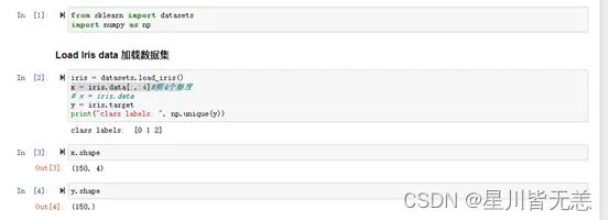
2、通过决策树算法对iris数据集总共四个维度的数据进行模型训练并求出错误率：

from sklearn import datasets
import numpy as np
iris = datasets.load_iris()
x = iris.data[:,:4]#前4个维度
# x = iris.data
y = iris.target
print("class labels: ", np.unique(y))
x.shape
y.shape

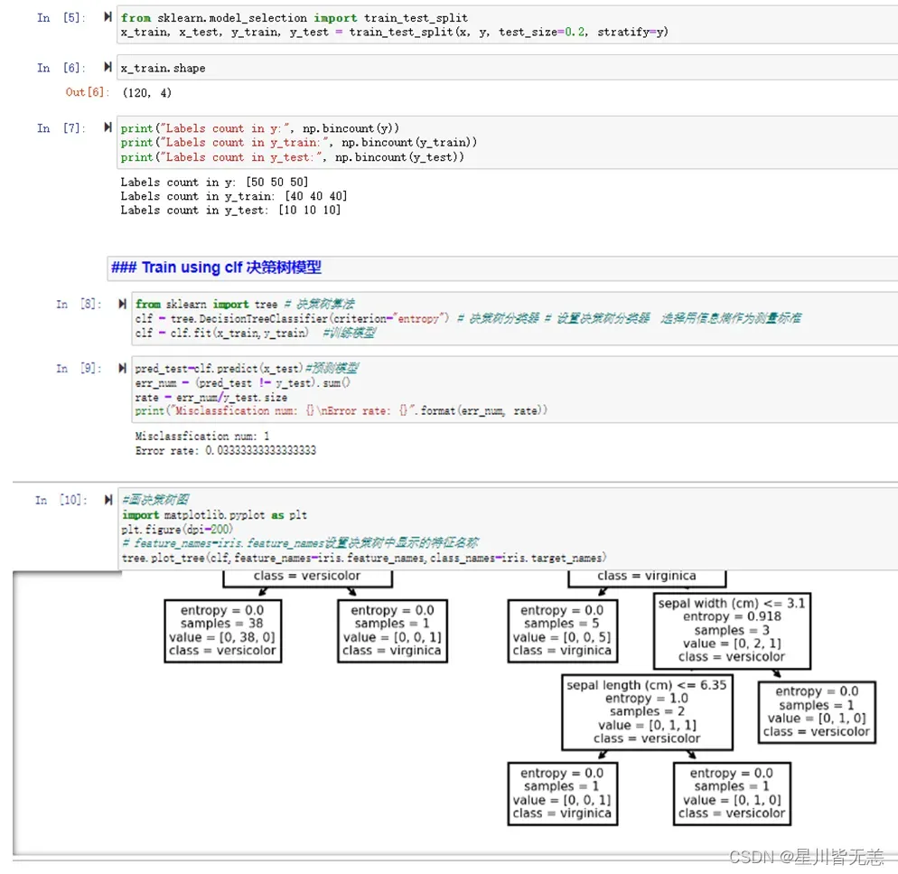
### split train and test sets 分割数据集和设置测试集
from sklearn.model_selection import train_test_split
x_train, x_test, y_train, y_test = train_test_split(x, y, test_size=0.2, stratify=y)
x_train.shape
print("Labels count in y:", np.bincount(y))
print("Labels count in y_train:", np.bincount(y_train))
print("Labels count in y_test:", np.bincount(y_test))

### Train using clf 决策树模型
from sklearn import tree # 决策树算法
clf = tree.DecisionTreeClassifier(criterion="entropy") # 决策树分类器 # 设置决策树分类器  选择用信息熵作为测量标准
clf = clf.fit(x_train,y_train)  #训练模型
pred_test=clf.predict(x_test)#预测模型
err_num = (pred_test != y_test).sum()
rate = err_num/y_test.size
print("Misclassfication num: {}\nError rate: {}".format(err_num, rate))

#画决策树图
import matplotlib.pyplot as plt
plt.figure(dpi=200)
# feature_names=iris.feature_names设置决策树中显示的特征名称
tree.plot_tree(clf,feature_names=iris.feature_names,class_names=iris.target_names)

代码运行截图

决策树算法既可以做分类也可以做回归，决策树也存在一些缺点，例如容易过拟合、对噪声数据敏感等。为了解决这些问题，我们可以对决策树进行剪枝或使用集成学习算法如随机森林来提高预测准确性。

过拟合是指模型在训练数据上表现很好，但在测试数据上表现不佳的现象。以下是一些解决决策树算法过拟合问题的方法：

剪枝：决策树剪枝是一种常用的方法，用于减少决策树的复杂度并避免过拟合。常见的剪枝方法包括预剪枝和后剪枝。预剪枝是在构建树时停止拆分某些节点，后剪枝是在构建完整的树之后，再去掉一些子树。
正则化：与其他机器学习算法一样，决策树也可以使用正则化技术来防止过拟合。例如，可以使用L1或L2正则化来约束树的复杂度。
随机化：通过引入随机化，可以减少决策树的方差并提高模型的鲁棒性。例如，可以在构建树时随机选择特征，而不是根据特定的规则进行选择。
集成学习：将多个决策树组合成一个集成模型，例如随机森林和梯度提升树等。这种方法可以通过减少单个决策树的方差来提高整体模型的泛化性能。
数据扩充：通过增加数据样本数量或改变数据样本的特征值，可以减少过拟合。例如，可以使用数据增强技术，如旋转、平移和缩放等来生成更多的训练样本。

祝各位五一劳动节快乐！

文章出处登录后可见！

已经登录？立即刷新