数据集来源UCI Machine Learning Repository: Abalone Data Set

一、数据集探索性分析

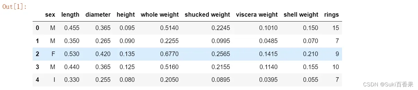
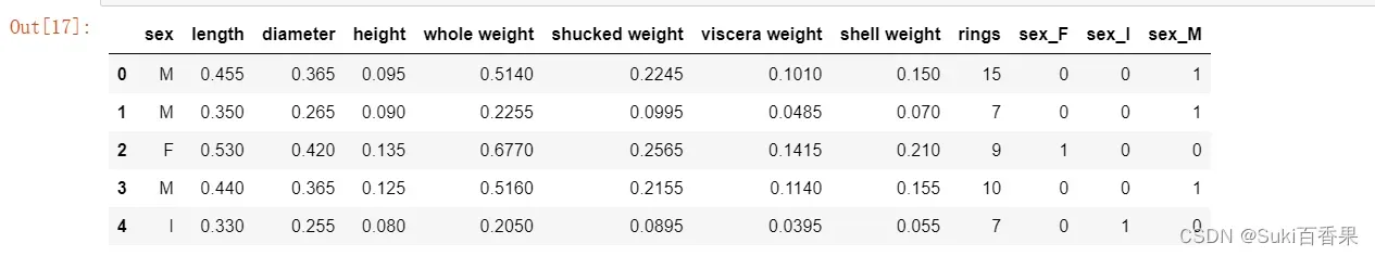
import pandas as pd
import numpy as np
import seaborn as sns
data = pd.read_csv("abalone_dataset.csv")
data.head()
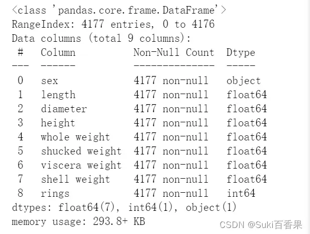
#查看数据集中样本数量和特征数量
data.shape
#查看数据信息，检查是否有缺失值
data.info()
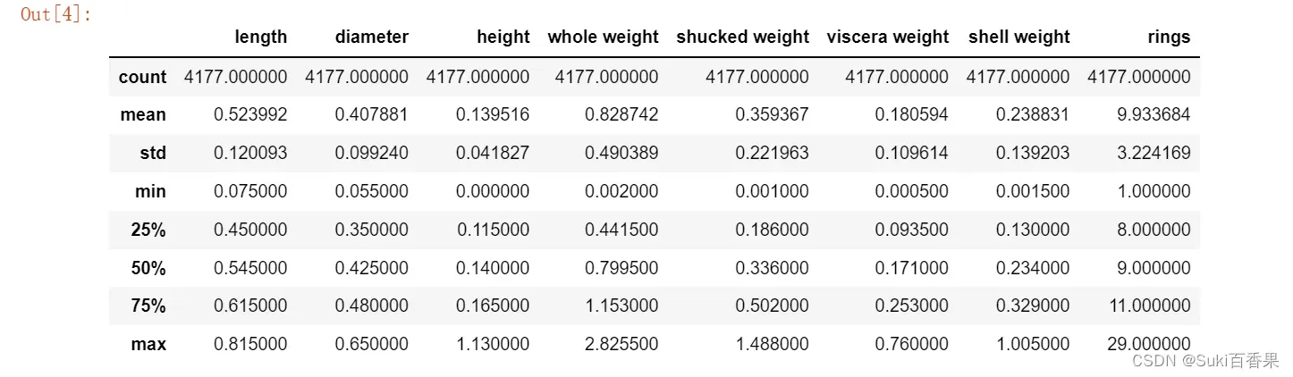
data.describe()
数据集一共有4177个样本，每个样本有9个特征。其中rings为鲍鱼环数，加上1.5等于鲍鱼年龄，是预测变量。除了sex为离散特征，其余都为连续变量。

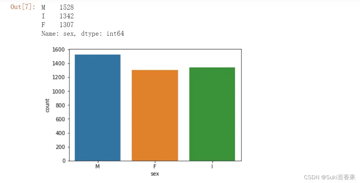
#观察sex列的取值分布情况
import numpy as np
import matplotlib.pyplot as plt
%matplotlib inline
sns.countplot(x='sex',data=data)
data['sex'].value_counts()

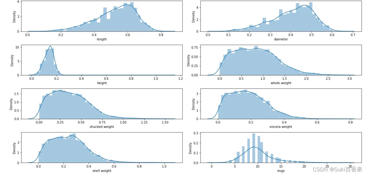
对于连续特征，可以使用seaborn的distplot函数绘制直方图观察特征取值情况。我们将8个连续特征的直方图绘制在一个4行2列的子图布局中。
i=1
plt.figure(figsize=(16,8))
for col in data.columns[1:]:
    plt.subplot(4,2,i)
    i=i+1
    sns.distplot(data[col])
plt.tight_layout()    

sns.pairplot()官网 seaborn.pairplot — seaborn 0.12.2 documentation
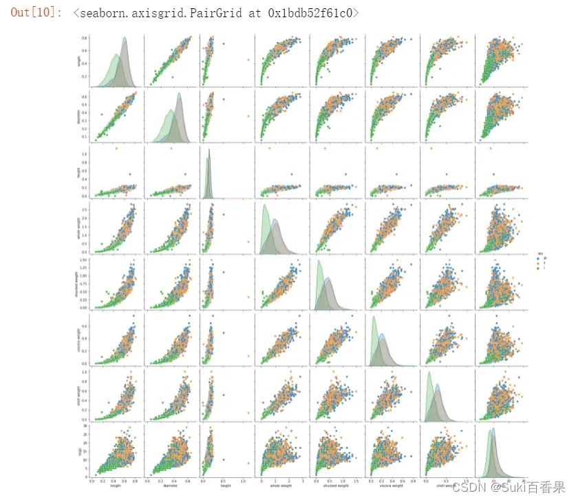
默认情况下，此函数将创建一个轴网格，这样数据中的每个数字变量将在单行的y轴和单列的x轴上共享。对角图的处理方式不同：绘制单变量分布图以显示每列数据的边际分布。也可以显示变量的子集或在行和列上绘制不同的变量。
#连续特征之间的散点图
sns.pairplot(data,hue='sex')
* 1.第一行观察得出：length和diameter、height存在明显的线性关系
* 2.最后一行观察得出：rings与各个特征均存在正相关性，其中与height的线性关系最为直观
* 3.对角线观察得出：sex“I”在各个特征取值明显小于成年鲍鱼

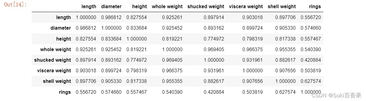
#计算特征之间的相关系数矩阵
corr_df = data.corr()
corr_df

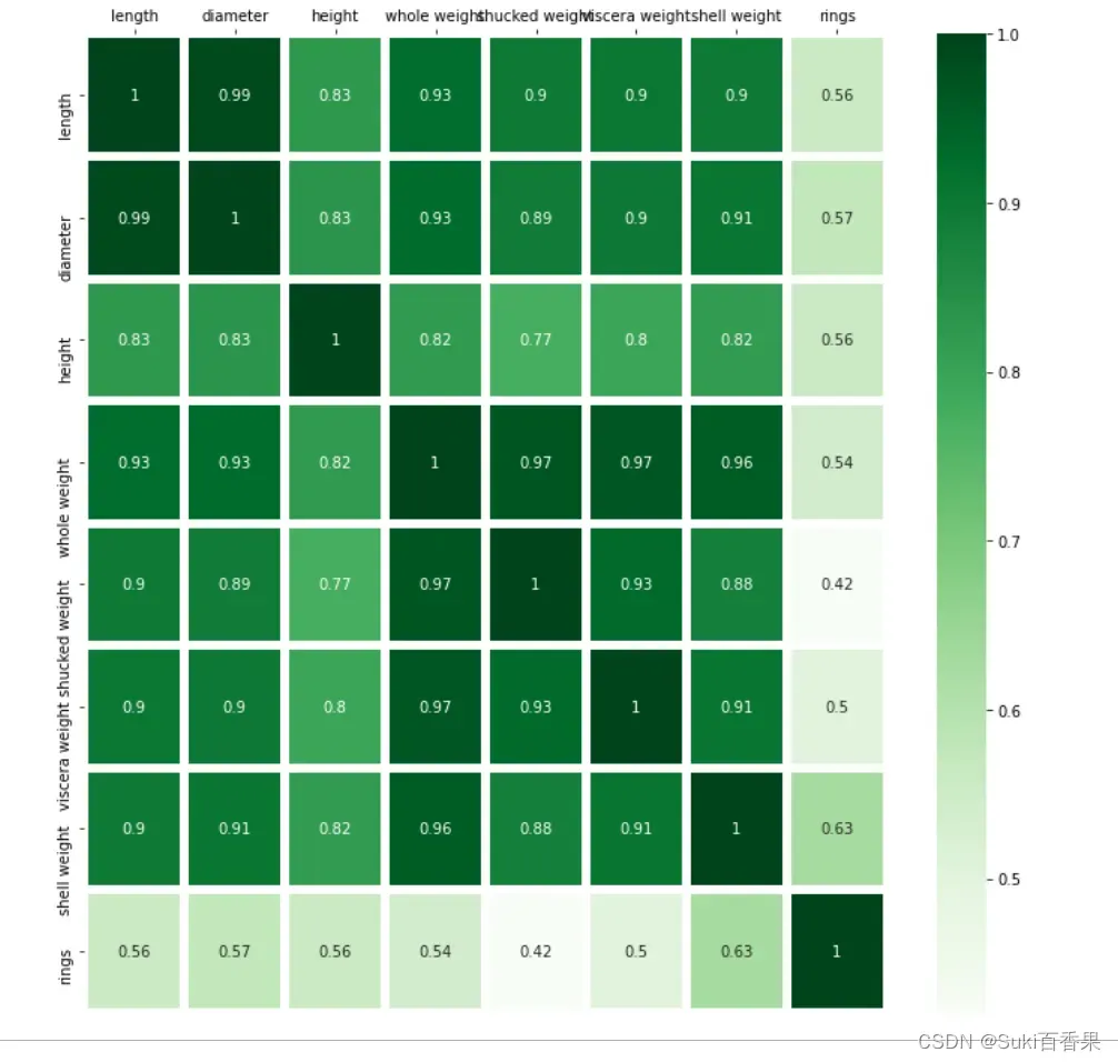
fig,ax =plt.subplots(figsize=(12,12))
#绘制热力图
ax = sns.heatmap(corr_df,linewidths=5,
                cmap='Greens',
                annot=True,
                xticklabels=corr_df.columns,
                yticklabels=corr_df.index)
ax.xaxis.set_label_position('top')
ax.xaxis.tick_top()

二、鲍鱼数据预处理

1.对sex特征进行OneHot编码，便于后续模型纳入哑变量

#类别变量--无先后之分，使用OneHot编码
#使用Pandas的get_dummies函数对sex特征做OneHot编码处理
sex_onehot =pd.get_dummies(data['sex'],prefix='sex')
#prefix--前缀
data[sex_onehot.columns] = sex_onehot
#将set_onehot加入data中
data.head()

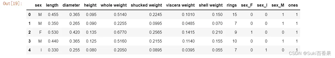
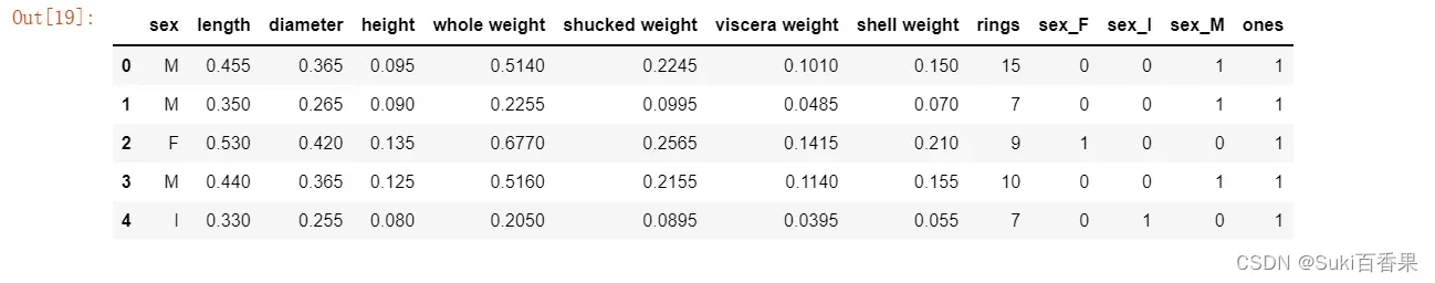
2.添加取值为1的特征

#截距项
data['ones']=1
data.head()

3. 计算鲍鱼的真实年龄

data["age"] =data['rings']+1.5
data.head()

4.筛选特征

多重共线性
*最小二乘的参数估计为 $\hat{w} =(X^{T}X)^{-1} X^{T} y$ 如果变量之间存在较强的共线性，则$X^TX$近似奇异，对参数的估计变得不准确，造成过度拟合现象。
*解决办法：正则化、主成分回归、偏最小二乘回归
所以sex_onehot的三列，线性相关，三列取两列选入x中

y=data['rings']
#不使用sklearn(包含ones)
features_with_ones=['length', 'diameter', 'height', 'whole weight', 'shucked weight',
       'viscera weight', 'shell weight', 'sex_F', 'sex_I','ones' ]
#使用sklearn（不包含ones）
features_without_ones=['length', 'diameter', 'height', 'whole weight', 'shucked weight',
       'viscera weight', 'shell weight', 'sex_F', 'sex_I']
X=data[features_with_ones]

5. 将鲍鱼数据集划分为训练集和测试集

#80%为训练集，20%为测试集
from sklearn.model_selection import train_test_split
X_train,X_test,y_train,y_test = train_test_split(X,y,test_size=0.2,random_state=111)

三、实现线性回归和岭回归

1. 使用Numpy使用线性回归

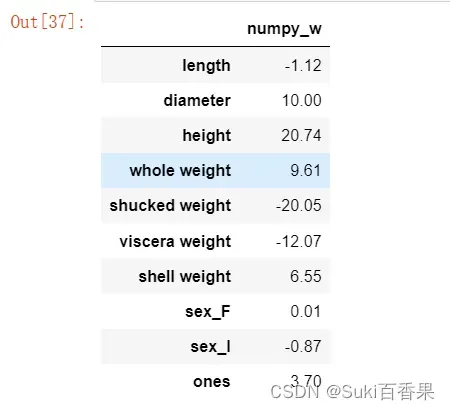
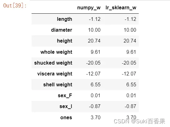
#判断xTx是否可逆，并计算得出w
#解析解求线性回归系数
def linear_regression(X,y):
    w = np.zeros_like(X.shape[1])
    if np.linalg.det(X.T.dot(X))!=0:
        w = np.linalg.inv(X.T.dot(X)).dot(X.T).dot(y)
    return w
#使用上述实现的线性回归模型在鲍鱼训练集上训练模型
w1=linear_regression(X_train,y_train)
w1 = pd.DataFrame(data=w1,index=X.columns,columns=['numpy_w'])
w1.round(decimals=2)
所以，求得的模型为
y=-1.12 * length + 10 * diameter + 20.74 * height + 9.61 * whole_weight – 20.05 * shucked_weight – 12.07 * viscera – weight + 6.55 * shell_weight + 0.01 * sex_F – 0.37 * sex_I + 3.70

2.使用Sklearn实现线性回归

from sklearn.linear_model import LinearRegression
lr = LinearRegression()
lr.fit(x_train[features_without_ones],y_train)
print(lr.coef_)

w_lr = []
w_lr.extend(lr.coef_)
w_lr.append(lr.intercept_)
w1['lr_sklearn_w']=w_lr
w1.round(decimals=2)

3.使用numpy实现岭回归

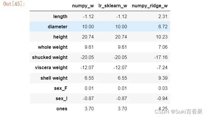
def ridge_regression(X,y,ridge_lambda):
    penalty_matrix = np.eye(X.shape[1])
    penalty_matrix[X.shape[1] - 1][X.shape[1] - 1] = 0
    w=np.linalg.inv(X.T.dot(X) + ridge_lambda*penalty_matrix).dot(X.T).dot(y)
    return w

$\hat{w} =(X^{T}X+\lambda X)^{-1} X^{T} y$

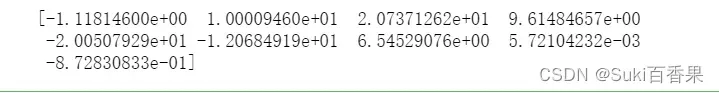
#正则化系数设置为1
w2 = ridge_regression(X_train,y_train,1.0)
print(w2)

w1['numpy_ridge_w']=w2
w1.round(decimals=2)

4. 利用sklearn实现岭回归

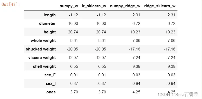
from sklearn.linear_model import Ridge
ridge = Ridge(alpha=1.0)
ridge.fit(X_train[features_without_ones],y_train)
w_ridge = []
w_ridge.extend(ridge.coef_)
w_ridge.append(ridge.intercept_)
w1["ridge_sklearn_w"] = w_ridge
w1.round(decimals=2)

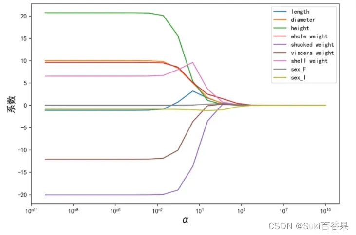
岭迹分析

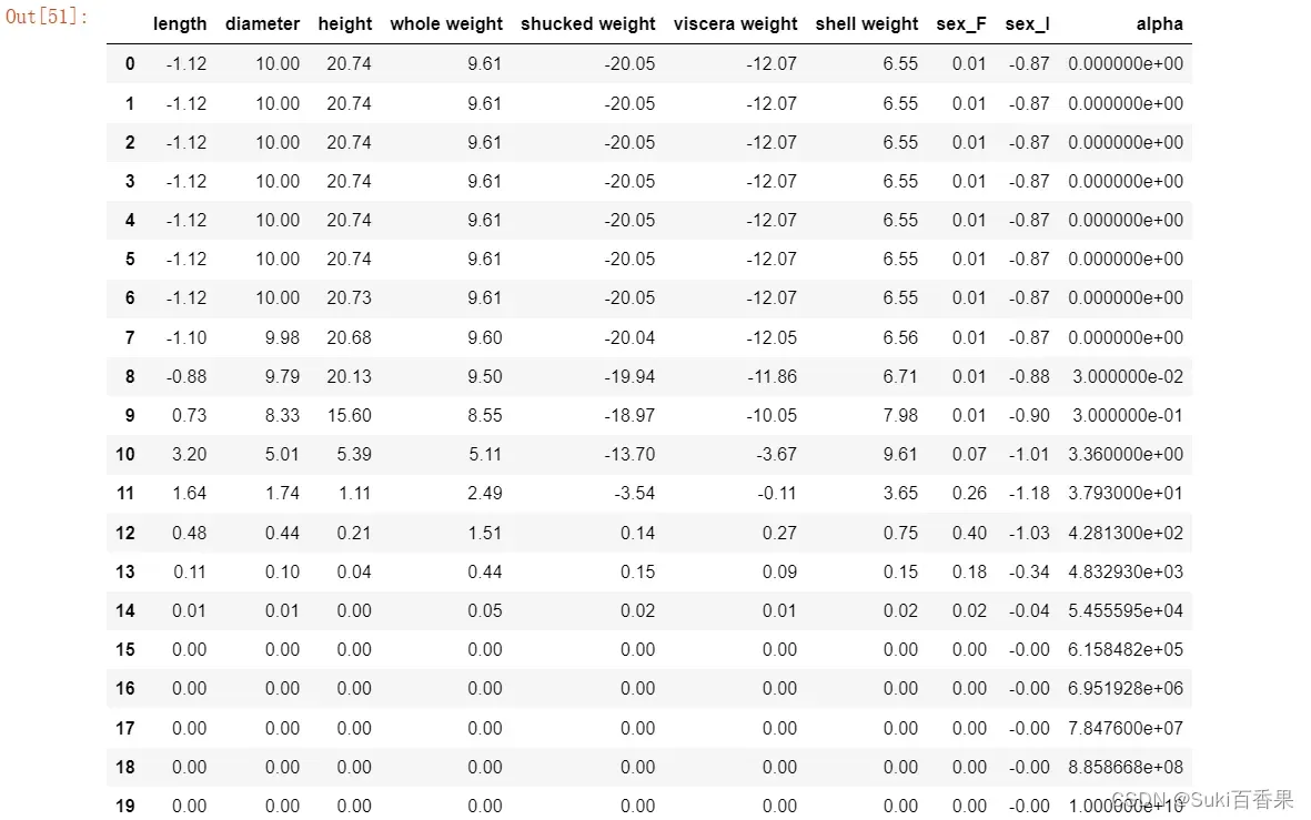
alphas = np.logspace(-10,10,20)
coef = pd.DataFrame()
for alpha in alphas:
    ridge_clf = Ridge(alpha=alpha)
    ridge_clf.fit(X_train[features_without_ones],y_train)
    df = pd.DataFrame([ridge_clf.coef_],columns=X_train[features_without_ones].columns)
    df['alpha']=alpha
    coef = coef.append(df,ignore_index=True)
coef.round(decimals=2)

import matplotlib.pyplot as plt
%matplotlib inline
#绘图
#显示中文和正负号
plt.rcParams['font.sans-serif']=['SimHei','Times New Roman']
plt.rcParams['axes.unicode_minus']=False
plt.rcParams['figure.dpi']=300#分辨率
plt.figure(figsize=(9,6))
coef['alpha']=coef['alpha']

for feature in X_train.columns[:-1]:
    plt.plot('alpha',feature,data=coef)
ax=plt.gca()
ax.set_xscale('log')
plt.legend(loc='upper right')
plt.xlabel(r'$\alpha$',fontsize=15)
plt.ylabel('系数',fontsize=15)

四、使用LASSO构建鲍鱼年龄预测模型

LASSO的目标函数

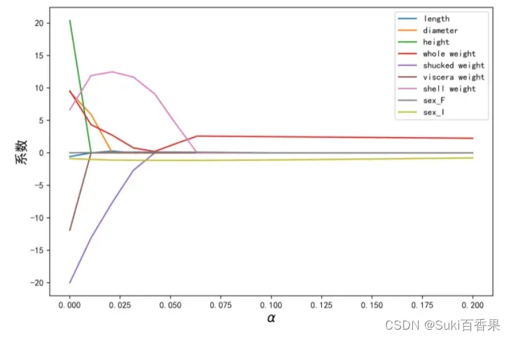
$(Xw-y)^T(Xw-y)+\lambda \parallel w\parallel _{1}$

随着𝜆增大，LASSO的特征系数逐个减小为0，可以做特征选择；而岭回归变量系数几乎趋近与0

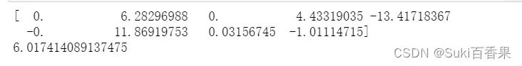
from sklearn.linear_model import Lasso
lasso=Lasso(alpha=0.01)
lasso.fit(X_train[features_without_ones],y_train)
print(lasso.coef_)
print(lasso.intercept_)

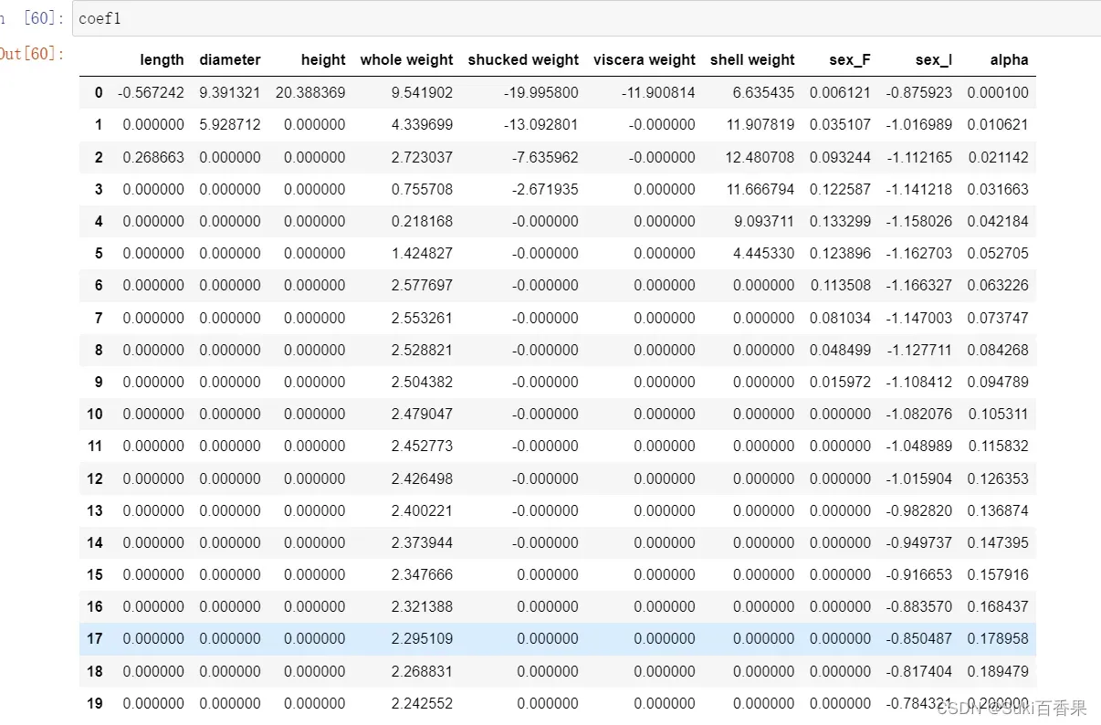
#LASSO的正则化渠道
coef1 = pd.DataFrame()
for alpha in np.linspace(0.0001,0.2,20):
    lasso_clf = Lasso(alpha=alpha)
    lasso_clf.fit(X_train[features_without_ones],y_train)
    df = pd.DataFrame([lasso_clf.coef_],columns=X_train[features_without_ones].columns)
    df['alpha']=alpha
    coef1 = coef1.append(df,ignore_index=True)
coef1.head()

plt.figure(figsize=(9,6),dpi=600)
for feature in X_train.columns[:-1]:
    plt.plot('alpha',feature,data=coef1)
plt.legend(loc='upper right')
plt.xlabel(r'$\alpha$',fontsize=15)
plt.ylabel('系数',fontsize=15)
plt.show()

coef1

五、鲍鱼年龄预测模型效果评估

1.计算MAE、MSE及R2系数

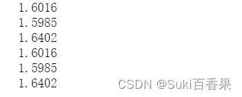
from sklearn.metrics import mean_squared_error
from sklearn.metrics import mean_absolute_error
from sklearn.metrics import r2_score
#MAE
y_test_pred_lr=lr.predict(X_test.iloc[:,:-1])
print(round(mean_absolute_error(y_test,y_test_pred_lr),4))

y_test_pred_ridge=ridge.predict(X_test[features_without_ones])
print(round(mean_absolute_error(y_test,y_test_pred_ridge),4))

y_test_pred_lasso=lasso.predict(X_test[features_without_ones])
print(round(mean_absolute_error(y_test,y_test_pred_lasso),4))

#MSE
y_test_pred_lr=lr.predict(X_test.iloc[:,:-1])
print(round(mean_absolute_error(y_test,y_test_pred_lr),4))

y_test_pred_ridge=ridge.predict(X_test[features_without_ones])
print(round(mean_absolute_error(y_test,y_test_pred_ridge),4))

y_test_pred_lasso=lasso.predict(X_test[features_without_ones])
print(round(mean_absolute_error(y_test,y_test_pred_lasso),4))

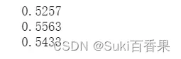
#R2系数
print(round(r2_score(y_test,y_test_pred_lr),4))
print(round(r2_score(y_test,y_test_pred_ridge),4))
print(round(r2_score(y_test,y_test_pred_lasso),4))

2.残差图

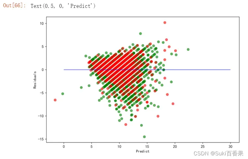
plt.figure(figsize=(9,6),dpi=600)
y_train_pred_ridge=ridge.predict(X_train[features_without_ones])
plt.scatter(y_train_pred_ridge,y_train_pred_ridge - y_train,c='g',alpha=0.6)
plt.scatter(y_test_pred_ridge,y_test_pred_ridge - y_test,c='r',alpha=0.6)
plt.hlines(y=0,xmin=0,xmax=30,color='b',alpha=0.6)
plt.ylabel('Residuals')
plt.xlabel('Predict')

观察残差图，可以发现测试集的点（红色）与训练集的点（绿点）基本吻合。模型训练效果不错。

文章出处登录后可见！

已经登录？立即刷新

鲍鱼数据集案例分析-预测鲍鱼年龄（线性回归/梯度下降法实操）