生成模型(四)：扩散模型02【第一单元：扩散模型简介】

第一单元：扩散模型简介

欢迎来到 Hugging Face 扩散模型课程第一单元！在本单元中，你将学习有关扩散模型如何工作的基础知识，以及如何使用 🤗 diffusers 库。

什么是扩散模型？

扩散模型是「生成模型」算法家族的新成员通过学习给定的训练样本，生成模型可以学会如何 生成 数据，比如生成图片或者声音。一个好的生成模型能生成一组 样式不同 的输出。这些输出会与训练数据相似，但不是一模一样的副本。扩散模型如何实现这一点？为了便于说明，让我们先看看图像生成的案例。

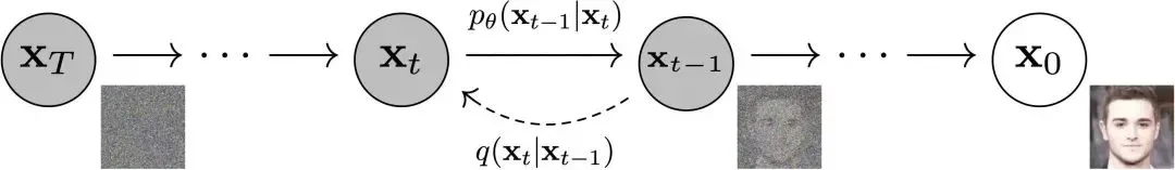
图片来源: DDPM paper (https://arxiv.org/abs/2006.11239)

扩散模型成功的秘诀在于扩散过程的迭代本质。最先生成的只是一组随机噪声，但经过若干步骤逐渐改善，有意义的图像将最终会出现。在每一步中，模型都会估计如何从当前的输入生成完全去噪的结果。因为我们在每一步都只做了一个小小的变动，所以在早期阶段（预测最终输出实际上非常困难），这个估计中的任何 error 都可以在以后的更新中得到纠正。

与其他类型的生成模型相比，训练扩散模型相对较为容易。我们只需要重复以下步骤即可：

1. 从训练数据中加载一些图像

2. 添加不同级别的噪声。请记住，我们希望模型在面对添加了极端噪声和几乎没有添加噪声的带噪图像时，都能够很好地估计如何「修复」(去噪)。

3. 将带噪输入送入模型中

4. 评估模型对这些输入进行去噪的效果

5. 使用此信息更新模型权重

为了用训练好的模型生成新的图像，我们从完全随机的输入开始，反复将其输入模型，每次根据模型预测进行少量更新。我们之后会学到有许多采样方法试图简化这个过程，以便我们可以用尽可能少的步骤生成好的图像。

我们将在第一单元的实践笔记本中详细介绍这些步骤。在第二单元中，我们将了解如何修改此过程，来通过额外的条件（例如类标签）或使用指导等技术来增加对模型输出的额外控制。第三单元和第四单元将探索一种非常强大的扩散模型，称为稳定扩散 (stable diffusion)，它可以生成给定文本描述的图像。

实践笔记本

到这里，您已经足够了解如何开始使用附带的笔记本了！这里的两个笔记本以不同的方式表达了相同的想法。

在 Diffuser 介绍 这个 Notebook 中，我们使用 diffusers 库中的构造模块显示了与上述不同的步骤。你将很快看到如何根据您选择的任何数据创建、训练和采样您自己的扩散模型。在笔记本结束时，您将能够阅读和修改示例训练脚本，以训练扩散模型，并将其与全世界共同分享！本笔记本还介绍了与本单元相关的主要练习，在这里，我们将共同尝试为不同规模的扩散模型找出好的「训练脚本」—— 请参阅下一节了解更多信息。

在 扩散模型从零到一 这个 Notebook 中，我们展示了相同的步骤（向数据添加噪声、创建模型、训练和采样），并尽可能简单地在 PyTorch 中从头开始实现。然后，我们将这个「玩具示例」与 diffusers 版本进行比较，并关注两者的区别以及改进之处。这里的目标是熟悉不同的组件和其中的设计决策，以便在查看新的实现时能够快速确定关键思想。我们也会在接下来的推送中发布这个 Notebook 的内容。

实践和分享

现在，你已经掌握了基本知识，可以开始训练你自己的扩散模型了！Diffuser 介绍 笔记本的末尾有一些小提示，希望您能与社区分享您的成果、训练脚本和发现，以便我们能够一起找出训练这些模型的最佳方法。

一些额外的材料

• 《Hugging Face 博客: 带注释的扩散模型》是对 DDPM 背后的代码和理论的非常深入的介绍，其中包括数学和显示了所有不同的组件的代码。它还链接了一些论文供进一步阅读:
  https://hf.co/blog/annotated-diffusion

• Hugging Face 文档: 无条件图像生成 (Unconditional Image-Generation)，包含了有关如何使用官方训练示例脚本训练扩散模型的一些示例，包括演示如何创建自己的数据集的代码：
  https://hf.co/docs/diffusers/training/unconditional_training

• AI Coffee Break video on Diffusion Models:
  https://www.youtube.com/watch?v=344w5h24-h8

• Yannic Kilcher Video on DDPMs:
  https://www.youtube.com/watch?v=W-O7AZNzbzQ

Diffuser 介绍 Notebook

在这个 Notebook 里，你将训练你的第一个扩散模型来 生成美丽的蝴蝶的图片 🦋。在此过程中，你将了解 🤗 Diffuers 库，它将为我们稍后将在课程中介绍的更高级的应用程序提供良好的基础

让我们开始吧！

你将学习到

• 看到一个强大的自定义扩散模型管道 (并了解到如何制作一个自己的版本)

• 通过以下方式创建你自己的迷你管道:

• 回顾扩散模型背后的核心思想

• 从 Hub 中加载数据进行训练

• 探索如何使用 scheduler 将噪声添加到数据中

• 创建和训练一个 UNet 模型

• 将各个组件拼装在一起来形成一个工作管道 (working pipelines)

• 编辑并运行一个脚本，用于初始化一个较长的训练，该脚本将处理

• 使用 Accelerate 来进行多 GPU 加速训练

• 实验日志记录以跟踪关键统计数据

• 将最终的模型上传到 Hugging Face Hub

❓如果你有任何问题，请发布在 Hugging Face 的 Discord 服务器#diffusion-models-class频道中。你可以在这里完成注册:
https://hf.co/join/discord

预备知识

在进入 Notebook 之前，你需要:

• 📖 阅读完上面的的材料

• 🤗 在 Hugging Face Hub 上创建一个账户。你可以在这里完成注册:
  https://hf.co/join

步骤 1: 设置

运行以下单元以安装 diffusers 库以及一些其他要求：

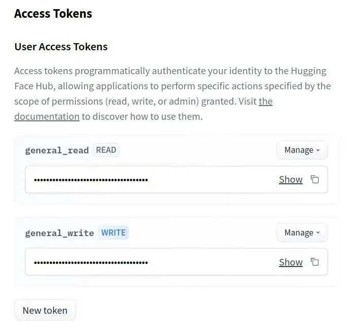
%pip install -qq -U diffusers datasets transformers accelerate ftfy pyarrow

接下来，请前往 https://huggingface.co/settings/tokens 创建具有写权限的访问令牌：

你可以使用命令行来通过此令牌登录 (huggingface-cli login) 或者运行以下单元来登录：

from huggingface_hub import notebook_login
notebook_login()

Login successful
Your token has been saved to /root/.huggingface/token

然后你需要安装 Git LFS 来上传模型检查点：

%%capture
!sudo apt -qq install git-lfs
!git config --global credential.helper store

最后，让我们导入将要使用的库，并定义一些方便函数，稍后我们将会在 Notebook 中使用这些函数：

import numpy as np
import torch
import torch.nn.functional as F
from matplotlib import pyplot as plt
from PIL import Image


def show_images (x):
   """Given a batch of images x, make a grid and convert to PIL"""
   x = x * 0.5 + 0.5  # Map from (-1, 1) back to (0, 1)
   grid = torchvision.utils.make_grid(x)
   grid_im = grid.detach().cpu().permute (1, 2, 0).clip (0, 1) * 255
   grid_im = Image.fromarray(np.array (grid_im).astype (np.uint8))
   return grid_im


def make_grid(images, size=64):
   """Given a list of PIL images, stack them together into a line for easy viewing"""
   output_im = Image.new("RGB", (size * len (images), size))
   for i, im in enumerate(images):
      output_im.paste(im.resize((size, size)), (i * size, 0))
   return output_im


# Mac users may need device = 'mps' (untested)
device = torch.device("cuda" if torch.cuda.is_available () else "cpu")

好了，我们都准备好了！

Dreambooth：即将到来的巅峰

如果你在过去几个月里看过人工智能相关的社交媒体，你就会听说过 Stable Diffusion 模型。这是一个强大的文本条件隐式扩散模型（别担心，我们将会学习这些概念）。但它有一个缺点：它不知道你或我长什么样，除非我们足够出名以至于互联网上发布我们的照片。

Dreambooth 允许我们创建自己的模型变体，并对特定的面部、对象或样式有一些额外的了解。Corridor Crew 制作了一段出色的视频，用一致的任务形象来讲故事，这是一个很好的说明了这种技术的能力的例子：

from IPython.display import YouTubeVideo
YouTubeVideo("W4Mcuh38wyM")

这是一个使用了一个名为「Mr Potato Head」的模型作为例子。该模型的训练使用了 5 张著名的儿童玩具 “Mr Potato Head”的照片。模型地址:
https://hf.co/sd-dreambooth-library/mr-potato-head

首先，让我们来加载这个管道。这些代码会自动从 Hub 下载模型权重等需要的文件。由于这个只有一行的 demo 需要下载数 GB 的数据，因此你可以跳过此单元格，只需欣赏样例输出即可！

from diffusers import StableDiffusionPipeline

# Check out https://hf.co/sd-dreambooth-library for loads of models from the community
model_id = "sd-dreambooth-library/mr-potato-head"

# Load the pipeline
pipe = StableDiffusionPipeline.from_pretrained(model_id, torch_dtype=torch.float16).to (
   device
)

Fetching 15 files:   0%|          | 0/15 [00:00

管道加载完成后，我们可以使用以下命令生成图像：

prompt = "an abstract oil painting of sks mr potato head by picasso"
image = pipe(prompt, num_inference_steps=50, guidance_scale=7.5).images[0]
image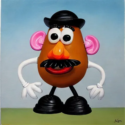

练习: 你可以使用不同的提示 (prompt) 自行尝试。在这个 demo 中，sks 是一个新概念的唯一标识符 (UID) – 那么如果把它留空的话会发生什么事呢？你还可以尝试改变 num_inference_steps 和 guidance_scale。这两个参数分别代表了采样步骤的数量（试试最多可以设为多低？）和模型将花多大的努力来尝试匹配提示。

这条神奇的管道里有很多事情！课程结束时，你将知道这一切是如何运作的。现在，让我们看看如何从头开始训练扩散模型。

MVP (最简可实行管道)

🤗 Diffusers 的核心 API 被分为三个主要部分:

1. 管道: 从高层出发设计的多种类函数，旨在以易部署的方式，能够做到快速通过主流预训练好的扩散模型来生成样本。

2. 模型: 训练新的扩散模型时用到的主流网络架构，举个例子 UNet:
   https://arxiv.org/abs/1505.04597

3. 管理器 (or 调度器): 在 推理 中使用多种不同的技巧来从噪声中生成图像，同时也可以生成在 训练 中所需的带噪图像。

管道对于末端使用者来说已经非常棒，但你既然已经参加了这门课程，我们就索性认为你想了解更多其中的奥秘！在此篇笔记结束之后，我们会来构建属于你自己，能够生成小蝴蝶图片的管道。下面这里会是最终的结果：

from diffusers import DDPMPipeline

# Load the butterfly pipeline
butterfly_pipeline = DDPMPipeline.from_pretrained(
   "johnowhitaker/ddpm-butterflies-32px"
).to (device)

# Create 8 images
images = butterfly_pipeline(batch_size=8).images

# View the result
make_grid(images)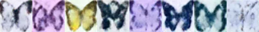

也许这看起来并不如 DreamBooth 所展示的样例那样惊艳，但要知道我们在训练这些图画时只用了不到训练稳定扩散模型用到数据的 0.0001%。说到模型训练，从引入介绍直到本单元，训练一个扩散模型的流程看起来像是这样：

1. 从训练集中加载一些图像

2. 加入噪声，从不同程度上

3. 把带了不同版本噪声的数据送进模型

4. 评估模型在对这些数据做增强去噪时的表现

5. 使用这个信息来更新模型权重，然后重复此步骤

我们会在接下来几节中逐一实现这些步骤，直至训练循环可以完整的运行，在这之后我们会来探索如何使用训练好的模型来生成样本，还有如何封装模型到管道中来轻松的分享给别人，下面我们来从数据入手吧。

步骤 2：下载一个训练数据集

在这个例子中，我们会用到一个来自 Hugging Face Hub 的图像集。具体来说，是个 1000 张蝴蝶图像收藏集。这是个非常小的数据集，我们这里也同时包含了已被注释的内容指向一些规模更大的选择。如果你想使用你自己的图像收藏，你也可以使用这里被注释掉的示例代码，从一个指定的文件夹来装载图片。

• 图像集地址:
  https://hf.co/datasets/huggan/smithsonian_butterflies_subset

import torchvision
from datasets import load_dataset
from torchvision import transforms

dataset = load_dataset("huggan/smithsonian_butterflies_subset", split="train")

# We'll train on 32-pixel square images, but you can try larger sizes too
image_size = 32
# You can lower your batch size if you're running out of GPU memory
batch_size = 64

# Define data augmentations
preprocess = transforms.Compose (
   [
      transforms.Resize((image_size, image_size)),  # Resize
      transforms.RandomHorizontalFlip(),  # Randomly flip (data augmentation)
      transforms.ToTensor(),  # Convert to tensor (0, 1)
      transforms.Normalize([0.5], [0.5]),  # Map to (-1, 1)
   ]
)


def transform(examples):
   images = [preprocess(image.convert("RGB")) for image in examples["image"]]
   return {"images": images}


dataset.set_transform(transform)

# Create a dataloader from the dataset to serve up the transformed images in batches
train_dataloader = torch.utils.data.DataLoader(
   dataset, batch_size=batch_size, shuffle=True
)

我们可以从中取出一批图像数据来看一看他们是什么样子:

xb = next(iter(train_dataloader))["images"].to(device)[:8]
print("X shape:", xb.shape)
show_images(xb).resize((8 * 64, 64), resample=Image.NEAREST)

X shape: torch.Size([8, 3, 32, 32])

/tmp/ipykernel_4278/3975082613.py:3: DeprecationWarning: NEAREST is deprecated and will be removed in Pillow 10 (2023-07-01). Use Resampling.NEAREST or Dither.NONE instead.
show_images (xb).resize ((8 * 64, 64), resample=Image.NEAREST)

我们在此篇 Notebook 中使用一个只有 32 像素的小图片集来保证训练时长是可控的。

步骤 3：定义管理器

我们的训练计划是，取出这些输入图片然后对它们增添噪声，在这之后把带噪的图片送入模型。在推理阶段，我们将用模型的预测值来不断迭代去除这些噪点。在 diffusers 中，这两个步骤都是由 管理器（调度器） 来处理的。

噪声管理器决定在不同的迭代周期时分别加入多少噪声。我们可以这样创建一个管理器，是取自于训练并能取样 ‘DDPM’ 的默认配置。基于此篇论文 Denoising Diffusion Probabalistic Models:
https://arxiv.org/abs/2006.11239

from diffusers import DDPMScheduler
noise_scheduler = DDPMScheduler(num_train_timesteps=1000)

DDPM 论文这样来描述一个损坏过程，为每一个「迭代周期」 (timestep) 增添一点少量的噪声。设在某个迭代周期有 , 我们可以得到它的下一个版本 （比之前更多一点点噪声）:

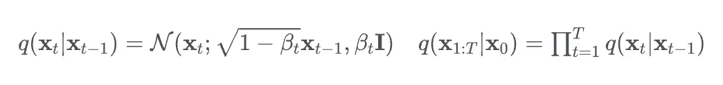
这就是说，我们取 , 给他一个 的系数，然后加上带有 系数的噪声。这里 是根据一些管理器来为每一个 t 设定的，来决定每一个迭代周期中添加多少噪声。现在，我们不想把这个推演进行 500 次来得到 ，所以我们用另一个公式来根据给出的 计算得到任意 t 时刻的 :

数学符号看起来总是很可怕！好在有管理器来为我们完成这些运算。我们可以画出 (标记为sqrt_alpha_prod) 和 (标记为sqrt_one_minus_alpha_prod) 来看一下输入 (x) 与噪声是如何在不同迭代周期中量化和叠加的:

plt.plot(noise_scheduler.alphas_cumprod.cpu() ** 0.5, label=r"${\sqrt {\bar {\alpha}_t}}$")
plt.plot((1 - noise_scheduler.alphas_cumprod.cpu()) ** 0.5, label=r"$\sqrt {(1 - \bar {\alpha}_t)}$")
plt.legend(fontsize="x-large");

练习: 你可以探索一下使用不同的 beta_start 时曲线是如何变化的，beta_end 与 beta_schedule 可以通过以下注释内容来修改:

# One with too little noise added:
# noise_scheduler = DDPMScheduler (num_train_timesteps=1000, beta_start=0.001, beta_end=0.004)
# The 'cosine' schedule, which may be better for small image sizes:
# noise_scheduler = DDPMScheduler (num_train_timesteps=1000, beta_schedule='squaredcos_cap_v2')

不论你选择了哪一个管理器 (调度器)，我们现在都可以使用 noise_scheduler.add_noise 功能来添加不同程度的噪声，就像这样：

timesteps = torch.linspace(0, 999, 8).long().to(device)
noise = torch.randn_like(xb)
noisy_xb = noise_scheduler.add_noise(xb, noise, timesteps)
print("Noisy X shape", noisy_xb.shape)
show_images (noisy_xb).resize((8 * 64, 64), resample=Image.NEAREST)

Noisy X shape torch.Size ([8, 3, 32, 32])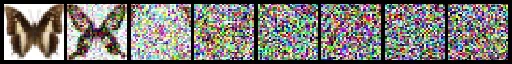

再来，在这里探索使用这里不同噪声管理器和预设参数带来的效果。这个视频很好的解释了一些上述数学运算的细节，同时也是对此类概念的一个很好引入介绍。视频地址:
https://www.youtube.com/watch?v=fbLgFrlTnGU

步骤 4：定义模型

现在我们来到了核心部分：模型本身。

大多数扩散模型使用的模型结构都是一些 U-net 的变形 (https://arxiv.org/abs/1505.04597)，也是我们在这里会用到的结构。

概括来说:

• 输入模型中的图片经过几个由 ResNetLayer 构成的层，其中每层都使图片尺寸减半。

• 之后在经过同样数量的层把图片升采样。

• 其中还有对特征在相同位置的上、下采样层残差连接模块。

模型一个关键特征既是，输出图片尺寸与输入图片相同，这正是我们这里需要的。

Diffusers 为我们提供了一个易用的UNet2DModel类，用来在 PyTorch 创建所需要的结构。

我们来使用 U-net 为我们生成目标大小的图片吧。注意这里down_block_types对应下采样模块 (上图中绿色部分), 而up_block_types对应上采样模块 (上图中红色部分):

from diffusers import UNet2DModel

# Create a model
model = UNet2DModel(
   sample_size=image_size,  # the target image resolution
   in_channels=3,  # the number of input channels, 3 for RGB images
   out_channels=3,  # the number of output channels
   layers_per_block=2,  # how many ResNet layers to use per UNet block
   block_out_channels=(64, 128, 128, 256),  # More channels -> more parameters
   down_block_types=(
      "DownBlock2D",  # a regular ResNet downsampling block
      "DownBlock2D",
      "AttnDownBlock2D",  # a ResNet downsampling block with spatial self-attention
      "AttnDownBlock2D",
),
   up_block_types=(
      "AttnUpBlock2D",
      "AttnUpBlock2D",  # a ResNet upsampling block with spatial self-attention
      "UpBlock2D",
      "UpBlock2D",  # a regular ResNet upsampling block
   ),
)
model.to(device);

当在处理更高分辨率的输入时，你可能想用更多层的下、上采样模块，让注意力层只聚焦在最低分辨率（最底）层来减少内存消耗。我们在之后会讨论该如何实验来找到最适用与你手头场景的配置方法。

我们可以通过输入一批数据和随机的迭代周期数来看输出是否与输入尺寸相同：

with torch.no_grad():
   model_prediction = model (noisy_xb, timesteps).sample
model_prediction.shape

torch.Size ([8, 3, 32, 32])

在下一步中，我们来看如何训练这个模型。

步骤 5：创建训练循环

终于可以训练了！下面这是 PyTorch 中经典的优化迭代循环，在这里一批一批的送入数据然后通过优化器来一步步更新模型参数 – 在这个样例中我们使用学习率为 0.0004 的 AdamW 优化器。

对于每一批的数据，我们要

• 随机取样几个迭代周期

• 根据预设为数据加入噪声

• 把带噪数据送入模型

• 使用 MSE 作为损失函数来比较目标结果与模型预测结果（在这里是加入噪声的场景）

• 通过loss.backward()与optimizer.step()来更新模型参数

在这个过程中我们记录 Loss 值用来后续的绘图。

NB: 这段代码大概需 10 分钟来运行 – 你也可以跳过以下两块操作直接使用预训练好的模型。供你选择，你可以探索下通过缩小模型层中的通道数会对运行速度有多少提升。

官方扩散模型示例训练了在更高分辨率数据集上的一个更大的模型，这也是一个极为精简训练循环的优秀示例，示例地址:
https://colab.research.google.com/github/huggingface/notebooks/blob/main/diffusers/training_example.ipynb

# Set the noise scheduler
noise_scheduler = DDPMScheduler (
   num_train_timesteps=1000, beta_schedule="squaredcos_cap_v2"
)

# Training loop
optimizer = torch.optim.AdamW(model.parameters (), lr=4e-4)

losses = []

for epoch in range(30):
   for step, batch in enumerate(train_dataloader):
      clean_images = batch["images"].to(device)
      # Sample noise to add to the images
      noise = torch.randn(clean_images.shape).to(clean_images.device)
      bs = clean_images.shape[0]

      # Sample a random timestep for each image
      timesteps = torch.randint (
      0, noise_scheduler.num_train_timesteps, (bs,), device=clean_images.device
      ).long()

      # Add noise to the clean images according to the noise magnitude at each timestep
      noisy_images = noise_scheduler.add_noise(clean_images, noise, timesteps)

      # Get the model prediction
      noise_pred = model(noisy_images, timesteps, return_dict=False)[0]

      # Calculate the loss
      loss = F.mse_loss(noise_pred, noise)
      loss.backward(loss)
      losses.append(loss.item())

      # Update the model parameters with the optimizer
      optimizer.step()
      optimizer.zero_grad()

   if (epoch + 1) % 5 == 0:
      loss_last_epoch = sum(losses [-len (train_dataloader) :]) /len (train_dataloader)
      print (f"Epoch:{epoch+1}, loss: {loss_last_epoch}")

Epoch:5, loss: 0.16273280512541533
Epoch:10, loss: 0.11161588924005628
Epoch:15, loss: 0.10206522420048714
Epoch:20, loss: 0.08302505919709802
Epoch:25, loss: 0.07805309211835265
Epoch:30, loss: 0.07474562455900013

绘制 loss 曲线，我们能看到模型在一开始快速的收敛，接下来以一个较慢的速度持续优化（我们用右边 log 坐标轴的视图可以看的更清楚）：

fig, axs = plt.subplots(1, 2, figsize=(12, 4))
axs [0].plot(losses)
axs [1].plot(np.log (losses))
plt.show()

[]

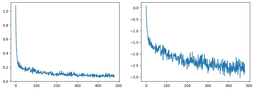
你可以选择运行上面的代码，也可以这样通过管道来调用模型：

# Uncomment to instead load the model I trained earlier:
# model = butterfly_pipeline.unet

步骤 6：生成图像

我们怎么从这个模型中得到图像呢？

方法 1：建立一个管道：

from diffusers import DDPMPipeline
image_pipe = DDPMPipeline(unet=model, scheduler=noise_scheduler)

pipeline_output = image_pipe()
pipeline_output.images[0]

0%|          | 0/1000 [00:00

我们可以在本地文件夹这样保存一个管道：

image_pipe.save_pretrained("my_pipeline")

检查文件夹的内容：

!ls my_pipeline/

model_index.json  scheduler  unet

这里scheduler与unet子文件夹中包含了生成图像所需的全部组件。比如，在unet文件中能看到模型参数 (diffusion_pytorch_model.bin) 与描述模型结构的配置文件。

!ls my_pipeline/unet/

config.json  diffusion_pytorch_model.bin

以上，这些文件包含了重新建立一个管道的全部内容。你可以手动把它们上传到 hub 来与他人分享你制作的管道，或使用下一节的 API 方法来记载。

方法 2：写一个取样循环

如果你去查看了管道中的 forward 方法，你可以看到在运行image_pipe()时发生了什么：

# ??image_pipe.forward

从随机噪声开始，遍历管理器的迭代周期来看从最嘈杂直到最微小的噪声变化，基于模型的预测一步步减少一些噪声：

# Random starting point (8 random images):
sample = torch.randn(8, 3, 32, 32).to(device)

for i, t in enumerate(noise_scheduler.timesteps):

   # Get model pred
   with torch.no_grad():
      residual = model(sample, t).sample

   # Update sample with step
   sample = noise_scheduler.step(residual, t, sample).prev_sample

show_images(sample)

noise_scheduler.step() 函数相应做了 sample（取样）时的数学运算。其实有很多取样的方法 – 在下一个单元我们将看到在已有模型的基础上如何换一个不同的取样器来加速图片生成，也会讲到更多从扩散模型中取样的背后原理。

步骤 7：把你的模型 Push 到 Hub

在上面的例子中我们把管道保存在了本地。把模型 push 到 hub 上，我们会需要建立模型和相应文件的仓库名。我们根据你的选择（模型 ID）来决定仓库的名字（大胆的去替换掉model_name吧；需要包含你的用户名，get_full_repo_name()会帮你做到）：

from huggingface_hub import get_full_repo_name

model_name = "sd-class-butterflies-32"
hub_model_id = get_full_repo_name(model_name)
hub_model_id

'lewtun/sd-class-butterflies-32'

然后，在 🤗 Hub 上创建模型仓库并 push 它吧：

from huggingface_hub import HfApi, create_repo

create_repo(hub_model_id)
api = HfApi()
api.upload_folder(
   folder_path="my_pipeline/scheduler", path_in_repo="", repo_id=hub_model_id
)
api.upload_folder(folder_path="my_pipeline/unet", path_in_repo="", repo_id=hub_model_id)
api.upload_file(
   path_or_fileobj="my_pipeline/model_index.json",
   path_in_repo="model_index.json",
   repo_id=hub_model_id,
)

'https://huggingface.co/lewtun/sd-class-butterflies-32/blob/main/model_index.json'

最后一件事是创建一个超棒的模型卡，如此，我们的蝴蝶生成器可以轻松的在 Hub 上被找到（请在描述中随意发挥！）：

from huggingface_hub import ModelCard

content = f"""
---
license: mit
tags:
- pytorch
- diffusers
- unconditional-image-generation
- diffusion-models-class
---

# Model Card for Unit 1 of the [Diffusion Models Class 🧨](https://github.com/huggingface/diffusion-models-class)

This model is a diffusion model for unconditional image generation of cute 🦋.

## Usage
```
python
from diffusers import DDPMPipeline

pipeline = DDPMPipeline.from_pretrained('{hub_model_id}')
image = pipeline ().images [0]
image
```
"""

card = ModelCard(content)
card.push_to_hub(hub_model_id)

现在模型已经在 Hub 上了，你可以这样从任何地方使用DDPMPipeline的from_pretrained()方法来下来它：

from diffusers import DDPMPipeline

image_pipe = DDPMPipeline.from_pretrained(hub_model_id)
pipeline_output = image_pipe()
pipeline_output.images[0]

Fetching 4 files:   0%|          | 0/4 [00:00

太棒了，成功了！

使用 🤗 Accelerate 来进行大规模使用

这篇笔记是用来教学，为此我尽力保证代码的简洁与轻量化。但也因为这样，我们也略去了一些内容你也许在使用更多数据训练一个更大的模式时，可能所需要用到的内容，如多块 GPU 支持，进度记录和样例图片，用于支持更大 batchsize 的导数记录功能，自动上传模型等等。好在这些功能大多数在这个示例代码中包含 here.

你可以这样下载该文件：

!wget https://github.com/huggingface/diffusers/raw/main/examples/unconditional_image_generation/train_unconditional.py

打开文件，你就可以看到模型是怎么定义的，以及有哪些可选的配置参数。我使用如下命令运行了该代码：

# Let's give our new model a name for the Hub
model_name = "sd-class-butterflies-64"
hub_model_id = get_full_repo_name(model_name)
hub_model_id

'lewtun/sd-class-butterflies-64'

!accelerate launch train_unconditional.py \
   --dataset_name="huggan/smithsonian_butterflies_subset"\
   --resolution=64 \
   --output_dir={model_name} \
   --train_batch_size=32 \
   --num_epochs=50 \
   --gradient_accumulation_steps=1 \
   --learning_rate=1e-4 \
   --lr_warmup_steps=500 \
   --mixed_precision="no"

如之前一样，把模型 push 到 hub，并且创建一个超酷的模型卡（按你的想法随意填写！）：

create_repo(hub_model_id)
api = HfApi()
api.upload_folder(
   folder_path=f"{model_name}/scheduler", path_in_repo="", repo_id=hub_model_id
)
api.upload_folder (
   folder_path=f"{model_name}/unet", path_in_repo="", repo_id=hub_model_id
)
api.upload_file (
   path_or_fileobj=f"{model_name}/model_index.json",
   path_in_repo="model_index.json",
   repo_id=hub_model_id,
)

content = f"""
---
license: mit
tags:
- pytorch
- diffusers
- unconditional-image-generation
- diffusion-models-class
---

# Model Card for Unit 1 of the [Diffusion Models Class 🧨](https://github.com/huggingface/diffusion-models-class)

This model is a diffusion model for unconditional image generation of cute 🦋.

## Usage
```
python
from diffusers import DDPMPipeline

pipeline = DDPMPipeline.from_pretrained ('{hub_model_id}')
image = pipeline ().images [0]
image
```
"""

card = ModelCard (content)
card.push_to_hub (hub_model_id)

'https://huggingface.co/lewtun/sd-class-butterflies-64/blob/main/README.md'

大概 45 分钟之后，得到这样的结果：

pipeline = DDPMPipeline.from_pretrained(hub_model_id).to (device)
images = pipeline(batch_size=8).images
make_grid(images)

0%|          | 0/1000 [00:00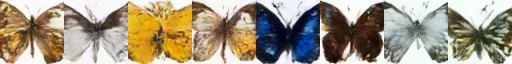

练习: 看看你能不能找到训练出在短时内能得到满意结果的模型训练设置参数，并与社群分享你的发现。阅读这些脚本看看你能不能理解它们，如果遇到了一些看上去令人迷惑的地方，请向大家提问来寻求解释。

更高阶的探索之路

希望这些能够让你初步了解可以使用 🤗 Diffusers library 来做什么！可能一些后续的步骤是这样：

• 尝试在新数据集上训练一个无限制的扩散模型 —— 如果你能直接自己完成那就太好了！你可以在 Hub 上的HugGan 社区小组页面找到一些能完成这个任务的超棒图像数据集。如果你不想等待模型训练太久的话，一定记得对图片做下采样！

• 创建自己的图片数据集：
  https://hf.co/docs/datasets/image_datase

• HugGan 社区小组页面：
  https://hf.co/huggan

• 试试用 DreamBooth 来创建你自己定制的扩散模型管道，请查看下面两个链接：

  Dreambooth Training Space 应用:
  https://hf.co/spaces/multimodalart/dreambooth-training

  Dreambooth fine-tuning for Stable Diffusion using d🧨ffusers 这个 Notebook:
  https://colab.research.google.com/github/huggingface/notebooks/blob/main/diffusers/sd_dreambooth_training.ipynb

• 修改训练脚本来探索使用不同的 UNet 超参数（层数深度，通道数等等），不同的噪声管理器等等。

扩散模型从零到一

这个 Notebook 我们将展示相同的步骤（向数据添加噪声、创建模型、训练和采样），并尽可能简单地在 PyTorch 中从头开始实现。然后，我们将这个「玩具示例」与 diffusers 版本进行比较，并关注两者的区别以及改进之处。这里的目标是熟悉不同的组件和其中的设计决策，以便在查看新的实现时能够快速确定关键思想。

让我们开始吧！

有时，只考虑一些事务最简单的情况会有助于更好地理解其工作原理。我们将在本笔记本中尝试这一点，从“玩具”扩散模型开始，看看不同的部分是如何工作的，然后再检查它们与更复杂的实现有何不同。

你将跟随本文的 Notebook 学习到

• 损坏过程（向数据添加噪声）

• 什么是 UNet，以及如何从零开始实现一个极小的 UNet

• 扩散模型训练

• 抽样理论

然后，我们将比较我们的版本与 diffusers 库中的 DDPM 实现的区别

• 对小型 UNet 的改进

• DDPM 噪声计划

• 训练目标的差异

• timestep 调节

• 抽样方法

这个笔记本相当深入，如果你对从零开始的深入研究不感兴趣，可以放心地跳过！

还值得注意的是，这里的大多数代码都是出于说明的目的，我不建议直接将其用于您自己的工作（除非您只是为了学习目的而尝试改进这里展示的示例）。

准备环境与导入：

!pip install -q diffusers

import torch
import torchvision
from torch import nn
from torch.nn import functional as F
from torch.utils.data import DataLoader
from diffusers import DDPMScheduler, UNet2DModel
from matplotlib import pyplot as plt

device = torch.device("cuda" if torch.cuda.is_available() else "cpu")
print(f'Using device: {device}')

数据

在这里，我们将使用一个非常小的经典数据集 mnist 来进行测试。如果您想在不改变任何其他内容的情况下给模型一个稍微困难一点的挑战，请使用 torchvision.dataset，FashionMNIST 应作为替代品。

dataset = torchvision.datasets.MNIST(root="mnist/", train=True, download=True, transform=torchvision.transforms.ToTensor())

train_dataloader = DataLoader(dataset, batch_size=8, shuffle=True)

x, y = next(iter(train_dataloader))
print('Input shape:', x.shape)
print('Labels:', y)
plt.imshow(torchvision.utils.make_grid(x)[0], cmap='Greys');

该数据集中的每张图都是一个数字的 28×28 像素的灰度图，像素值的范围是从 0 到 1。

损坏过程

假设你没有读过任何扩散模型的论文，但你知道这个过程会增加噪声。你会怎么做？

我们可能想要一个简单的方法来控制损坏的程度。那么，如果我们要引入一个参数来控制输入的“噪声量”，那么我们会这么做：

noise = torch.rand_like(x)

noisy_x = (1-amount)*x + amount*noise

如果 amount = 0，则返回输入而不做任何更改。如果 amount = 1，我们将得到一个纯粹的噪声。通过这种方式将输入与噪声混合，我们将输出保持在相同的范围（0 to 1）。

我们可以很容易地实现这一点（但是要注意 tensor 的 shape，以防被广播 (broadcasting) 机制不正确的影响到）：

def corrupt(x, amount):
  """Corrupt the input `x` by mixing it with noise according to `amount`"""
  noise = torch.rand_like(x)
  amount = amount.view(-1, 1, 1, 1) # Sort shape so broadcasting works
  return x*(1-amount) + noise*amount

让我们来可视化一下输出的结果，以了解是否符合我们的预期：

# Plotting the input data
fig, axs = plt.subplots(2, 1, figsize=(12, 5))
axs[0].set_title('Input data')
axs[0].imshow(torchvision.utils.make_grid(x)[0], cmap='Greys')

# Adding noise
amount = torch.linspace(0, 1, x.shape[0]) # Left to right -> more corruption
noised_x = corrupt(x, amount)

# Plottinf the noised version
axs[1].set_title('Corrupted data (-- amount increases -->)')
axs[1].imshow(torchvision.utils.make_grid(noised_x)[0], cmap='Greys');

当噪声量接近 1 时，我们的数据开始看起来像纯随机噪声。但对于大多数的噪声情况下，您还是可以很好地识别出数字。你认为这是最佳的吗？

模型

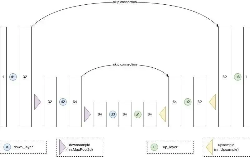
我们想要一个模型，它可以接收 28px 的噪声图像，并输出相同形状的预测。一个比较流行的选择是一个叫做 UNet 的架构。最初被发明用于医学图像中的分割任务，UNet 由一个“压缩路径”和一个“扩展路径”组成。“压缩路径”会使通过该路径的数据被压缩，而通过“扩展路径”会将数据扩展回原始维度（类似于自动编码器）。模型中的残差连接也允许信息和梯度在不同层级之间流动。

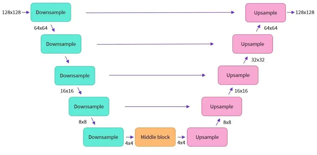
一些 UNet 的设计在每个阶段都有复杂的 blocks，但对于这个玩具 demo，我们只会构建一个最简单的示例，它接收一个单通道图像，并通过下行路径上的三个卷积层（图和代码中的 down_layers）和上行路径上的 3 个卷积层，在下行和上行层之间具有残差连接。我们将使用 max pooling 进行下采样和 nn.Upsample 用于上采样。某些比较复杂的 UNets 的设计会使用带有可学习参数的上采样和下采样 layer。下面的结构图大致展示了每个 layer 的输出通道数：

代码实现如下：

class BasicUNet(nn.Module):
  """A minimal UNet implementation."""
  def __init__(self, in_channels=1, out_channels=1):
    super().__init__()
    self.down_layers = torch.nn.ModuleList([ 
      nn.Conv2d(in_channels, 32, kernel_size=5, padding=2),
      nn.Conv2d(32, 64, kernel_size=5, padding=2),
      nn.Conv2d(64, 64, kernel_size=5, padding=2),
    ])
    self.up_layers = torch.nn.ModuleList([
      nn.Conv2d(64, 64, kernel_size=5, padding=2),
      nn.Conv2d(64, 32, kernel_size=5, padding=2),
      nn.Conv2d(32, out_channels, kernel_size=5, padding=2), 
    ])
    self.act = nn.SiLU() # The activation function
    self.downscale = nn.MaxPool2d(2)
    self.upscale = nn.Upsample(scale_factor=2)

  def forward(self, x):
    h = []
    for i, l in enumerate(self.down_layers):
      x = self.act(l(x)) # Through the layer n the activation function
      if i < 2: # For all but the third (final) down layer:
        h.append(x) # Storing output for skip connection
        x = self.downscale(x) # Downscale ready for the next layer
              
    for i, l in enumerate(self.up_layers):
      if i > 0: # For all except the first up layer
        x = self.upscale(x) # Upscale
        x += h.pop() # Fetching stored output (skip connection)
        x = self.act(l(x)) # Through the layer n the activation function
            
    return x

我们可以验证输出 shape 是否如我们期望的那样与输入相同：

net = BasicUNet()
x = torch.rand(8, 1, 28, 28)
net(x).shape

torch.Size([8, 1, 28, 28])

该网络有 30 多万个参数：

sum([p.numel() for p in net.parameters()])

309057

您可以尝试更改每个 layer 中的通道数或尝试不同的结构设计。

训练模型

那么，模型到底应该做什么呢？同样，对这个问题有各种不同的看法，但对于这个演示，让我们选择一个简单的框架：给定一个损坏的输入 noisy_x，模型应该输出它对原本 x 的最佳猜测。我们将通过均方误差将预测与真实值进行比较。

我们现在可以尝试训练网络了。

• 获取一批数据

• 添加随机噪声

• 将数据输入模型

• 将模型预测与干净图像进行比较，以计算 loss

• 更新模型的参数

你可以自由进行修改来尝试获得更好的结果！

# Dataloader (you can mess with batch size)
batch_size = 128
train_dataloader = DataLoader(dataset, batch_size=batch_size, shuffle=True)

# How many runs through the data should we do?
n_epochs = 3

# Create the network
net = BasicUNet()
net.to(device)

# Our loss finction
loss_fn = nn.MSELoss()

# The optimizer
opt = torch.optim.Adam(net.parameters(), lr=1e-3) 

# Keeping a record of the losses for later viewing
losses = []

# The training loop
for epoch in range(n_epochs):

  for x, y in train_dataloader:
    # Get some data and prepare the corrupted version
    x = x.to(device) # Data on the GPU
    noise_amount = torch.rand(x.shape[0]).to(device) # Pick random noise amounts
    noisy_x = corrupt(x, noise_amount) # Create our noisy x

    # Get the model prediction
    pred = net(noisy_x)

    # Calculate the loss
    loss = loss_fn(pred, x) # How close is the output to the true 'clean' x?

    # Backprop and update the params:
    opt.zero_grad()
    loss.backward()
    opt.step()

    # Store the loss for later
    losses.append(loss.item())

    # Print our the average of the loss values for this epoch:
    avg_loss = sum(losses[-len(train_dataloader):])/len(train_dataloader)
    print(f'Finished epoch {epoch}. Average loss for this epoch: {avg_loss:05f}')

# View the loss curve
plt.plot(losses)
plt.ylim(0, 0.1);

Finished epoch 0. Average loss for this epoch: 0.026736
Finished epoch 1. Average loss for this epoch: 0.020692
Finished epoch 2. Average loss for this epoch: 0.018887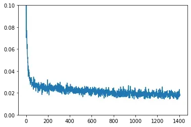

我们可以尝试通过抓取一批数据，以不同的数量损坏数据，然后喂进模型获得预测来观察结果：

#@markdown Visualizing model predictions on noisy inputs:

# Fetch some data
x, y = next(iter(train_dataloader))
x = x[:8] # Only using the first 8 for easy plotting

# Corrupt with a range of amounts
amount = torch.linspace(0, 1, x.shape[0]) # Left to right -> more corruption
noised_x = corrupt(x, amount)

# Get the model predictions
with torch.no_grad():
  preds = net(noised_x.to(device)).detach().cpu()

# Plot
fig, axs = plt.subplots(3, 1, figsize=(12, 7))
axs[0].set_title('Input data')
axs[0].imshow(torchvision.utils.make_grid(x)[0].clip(0, 1), cmap='Greys')
axs[1].set_title('Corrupted data')
axs[1].imshow(torchvision.utils.make_grid(noised_x)[0].clip(0, 1), cmap='Greys')
axs[2].set_title('Network Predictions')
axs[2].imshow(torchvision.utils.make_grid(preds)[0].clip(0, 1), cmap='Greys');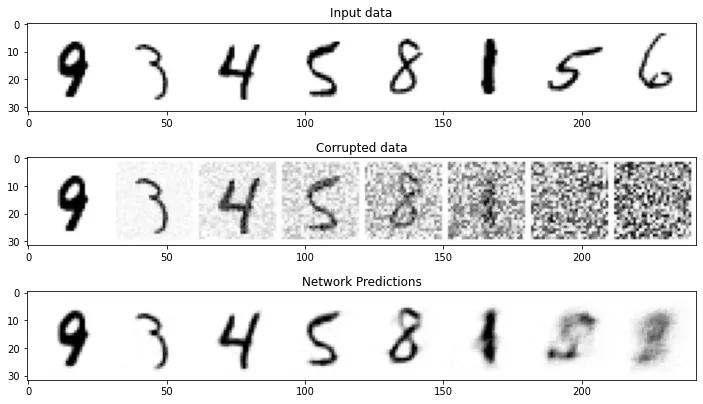

你可以看到，对于较低的噪声水平数量，预测的结果相当不错！但是，当噪声水平非常高时，模型能够获得的信息就开始逐渐减少。而当我们达到 amount = 1 时，模型会输出一个模糊的预测，该预测会很接近数据集的平均值。模型通过这样的方式来猜测原始输入。

取样（采样）

如果我们在高噪声水平下的预测不是很好，我们如何才能生成图像呢？

如果我们从完全随机的噪声开始，检查一下模型预测的结果，然后只朝着预测方向移动一小部分，比如说 20%。现在我们有一个噪声很多的图像，其中可能隐藏了一些关于输入数据的结构的提示，我们可以将其输入到模型中以获得新的预测。希望这个新的预测比第一个稍微好一点（因为我们这一次的输入稍微减少了一点噪声），所以我们可以用这个新的更好的预测再往前迈出一小步。

如果一切顺利的话，以上过程重复几次以后我们就会得到一个新的图像！以下图例是迭代了五次以后的结果，左侧是每个阶段的模型输入的可视化，右侧则是预测的去噪图像。请注意，即使模型在第 1 步就预测了去噪图像，我们也只是将输入向去噪图像变换了一小部分。重复几次以后，图像的结构开始逐渐出现并得到改善 , 直到获得我们的最终结果为止。

#@markdown Sampling strategy: Break the process into 5 steps and move 1/5'th of the way there each time:
n_steps = 5
x = torch.rand(8, 1, 28, 28).to(device) # Start from random
step_history = [x.detach().cpu()]
pred_output_history = []

for i in range(n_steps):
  with torch.no_grad(): # No need to track gradients during inference
    pred = net(x) # Predict the denoised x0
  pred_output_history.append(pred.detach().cpu()) # Store model output for plotting
  mix_factor = 1/(n_steps - i) # How much we move towards the prediction
  x = x*(1-mix_factor) + pred*mix_factor # Move part of the way there
  step_history.append(x.detach().cpu()) # Store step for plotting

fig, axs = plt.subplots(n_steps, 2, figsize=(9, 4), sharex=True)
axs[0,0].set_title('x (model input)')
axs[0,1].set_title('model prediction')
for i in range(n_steps):
  axs[i, 0].imshow(torchvision.utils.make_grid(step_history[i])[0].clip(0, 1), cmap='Greys')
  axs[i, 1].imshow(torchvision.utils.make_grid(pred_output_history[i])[0].clip(0, 1), cmap='Greys')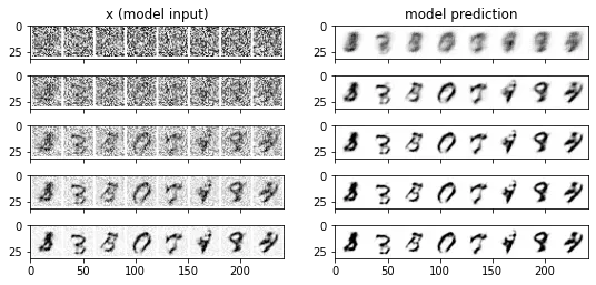

我们可以将流程分成更多步骤，并希望通过这种方式获得更好的图像：

#@markdown Showing more results, using 40 sampling steps
n_steps = 40
x = torch.rand(64, 1, 28, 28).to(device)
for i in range(n_steps):
  noise_amount = torch.ones((x.shape[0], )).to(device) * (1-(i/n_steps)) # Starting high going low
  with torch.no_grad():
    pred = net(x)
  mix_factor = 1/(n_steps - i)
  x = x*(1-mix_factor) + pred*mix_factor
fig, ax = plt.subplots(1, 1, figsize=(12, 12))
ax.imshow(torchvision.utils.make_grid(x.detach().cpu(), nrow=8)[0].clip(0, 1), cmap='Greys')

<matplotlib.image.AxesImage at 0x7f27567d8210>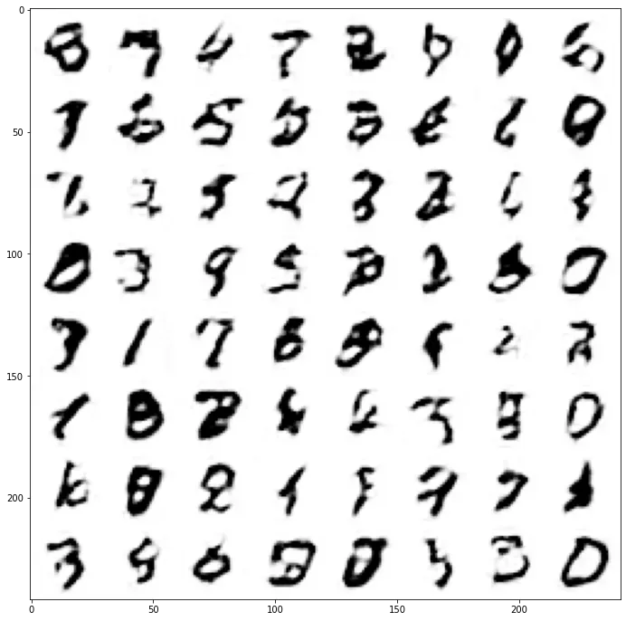

结果并不是非常好，但是已经出现了一些可以被认出来的数字！您可以尝试训练更长时间（例如，10 或 20 个 epoch），并调整模型配置、学习率、优化器等。此外，如果您想尝试稍微困难一点的数据集，您可以尝试一下 fashionMNIST，只需要一行代码的替换就可以了。

与 DDPM 做比较

在本节中，我们将看看我们的“玩具”实现与其他笔记本中使用的基于 DDPM 论文的方法有何不同: 扩散器简介 Notebook。

• 扩散器简介 Notebook:
  https://github.com/huggingface/diffusion-models-class/blob/main/unit1/01_introduction_to_diffusers.ipynb

我们将会看到的

• 模型的表现受限于随迭代周期 (timesteps) 变化的控制条件，在前向传导中时间步 (t) 是作为一个参数被传入的

• 有很多不同的取样策略可选择，可能会比我们上面所使用的最简单的版本更好

• diffusers UNet2DModel 比我们的 BasicUNet 更先进

• 损坏过程的处理方式不同

• 训练目标不同，包括预测噪声而不是去噪图像

• 该模型通过调节 timestep 来调节噪声水平 , 其中 t 作为一个附加参数传入前向过程中。

• 有许多不同的采样策略可供选择，它们应该比我们上面简单的版本更有效。

自 DDPM 论文发表以来，已经有人提出了许多改进建议，但这个例子对于不同的可用设计决策具有指导意义。读完这篇文章后，你可能会想要深入了解这篇论文《Elucidating the Design Space of Diffusion-Based Generative Models》，它对所有这些组件进行了详细的探讨，并就如何获得最佳性能提出了新的建议。

Elucidating the Design Space of Diffusion-Based Generative Models 论文链接:
https://arxiv.org/abs/2206.00364

如果你觉得这些内容对你来说太过深奥了，请不要担心！你可以随意跳过本笔记本的其余部分或将其保存以备不时之需。

UNet

diffusers 中的 UNet2DModel 模型比上述基本 UNet 模型有许多改进：

• GroupNorm 层对每个 blocks 的输入进行了组标准化（group normalization）

• Dropout 层能使训练更平滑

• 每个块有多个 resnet 层（如果 layers_per_block 未设置为 1）

• 注意机制（通常仅用于输入分辨率较低的 blocks）

• timestep 的调节。

• 具有可学习参数的下采样和上采样块

让我们来创建并仔细研究一下 UNet2DModel：

model = UNet2DModel(
  sample_size=28,           # the target image resolution
  in_channels=1,            # the number of input channels, 3 for RGB images
  out_channels=1,           # the number of output channels
  layers_per_block=2,       # how many ResNet layers to use per UNet block
  block_out_channels=(32, 64, 64), # Roughly matching our basic unet example
  down_block_types=( 
    "DownBlock2D",        # a regular ResNet downsampling block
    "AttnDownBlock2D",    # a ResNet downsampling block w/ spatial self-attention
    "AttnDownBlock2D",
  ), 
  up_block_types=(
    "AttnUpBlock2D", 
    "AttnUpBlock2D",      # a ResNet upsampling block with spatial self-attention
    "UpBlock2D",          # a regular ResNet upsampling block
  ),
)
print(model)

UNet2DModel(
  (conv_in): Conv2d(1, 32, kernel_size=(3, 3), stride=(1, 1), padding=(1, 1))
  (time_proj): Timesteps()
  (time_embedding): TimestepEmbedding(
    (linear_1): Linear(in_features=32, out_features=128, bias=True)
    (act): SiLU()
    (linear_2): Linear(in_features=128, out_features=128, bias=True)
  )
  (down_blocks): ModuleList(
    (0): DownBlock2D(
      (resnets): ModuleList(
        (0): ResnetBlock2D(
          (norm1): GroupNorm(32, 32, eps=1e-05, affine=True)
          (conv1): Conv2d(32, 32, kernel_size=(3, 3), stride=(1, 1), padding=(1, 1))
          (time_emb_proj): Linear(in_features=128, out_features=32, bias=True)
          (norm2): GroupNorm(32, 32, eps=1e-05, affine=True)
          (dropout): Dropout(p=0.0, inplace=False)
          (conv2): Conv2d(32, 32, kernel_size=(3, 3), stride=(1, 1), padding=(1, 1))
          (nonlinearity): SiLU()
        )
        (1): ResnetBlock2D(
          (norm1): GroupNorm(32, 32, eps=1e-05, affine=True)
          (conv1): Conv2d(32, 32, kernel_size=(3, 3), stride=(1, 1), padding=(1, 1))
          (time_emb_proj): Linear(in_features=128, out_features=32, bias=True)
          (norm2): GroupNorm(32, 32, eps=1e-05, affine=True)
          (dropout): Dropout(p=0.0, inplace=False)
          (conv2): Conv2d(32, 32, kernel_size=(3, 3), stride=(1, 1), padding=(1, 1))
          (nonlinearity): SiLU()
        )
      )
      (downsamplers): ModuleList(
        (0): Downsample2D(
          (conv): Conv2d(32, 32, kernel_size=(3, 3), stride=(2, 2), padding=(1, 1))
        )
      )
    )
    (1): AttnDownBlock2D(
      (attentions): ModuleList(
        (0): AttentionBlock(
          (group_norm): GroupNorm(32, 64, eps=1e-05, affine=True)
          (query): Linear(in_features=64, out_features=64, bias=True)
          (key): Linear(in_features=64, out_features=64, bias=True)
          (value): Linear(in_features=64, out_features=64, bias=True)
          (proj_attn): Linear(in_features=64, out_features=64, bias=True)
        )
        (1): AttentionBlock(
          (group_norm): GroupNorm(32, 64, eps=1e-05, affine=True)
          (query): Linear(in_features=64, out_features=64, bias=True)
          (key): Linear(in_features=64, out_features=64, bias=True)
          (value): Linear(in_features=64, out_features=64, bias=True)
          (proj_attn): Linear(in_features=64, out_features=64, bias=True)
        )
      )
      (resnets): ModuleList(
        (0): ResnetBlock2D(
          (norm1): GroupNorm(32, 32, eps=1e-05, affine=True)
          (conv1): Conv2d(32, 64, kernel_size=(3, 3), stride=(1, 1), padding=(1, 1))
          (time_emb_proj): Linear(in_features=128, out_features=64, bias=True)
          (norm2): GroupNorm(32, 64, eps=1e-05, affine=True)
          (dropout): Dropout(p=0.0, inplace=False)
          (conv2): Conv2d(64, 64, kernel_size=(3, 3), stride=(1, 1), padding=(1, 1))
          (nonlinearity): SiLU()
          (conv_shortcut): Conv2d(32, 64, kernel_size=(1, 1), stride=(1, 1))
        )
        (1): ResnetBlock2D(
          (norm1): GroupNorm(32, 64, eps=1e-05, affine=True)
          (conv1): Conv2d(64, 64, kernel_size=(3, 3), stride=(1, 1), padding=(1, 1))
          (time_emb_proj): Linear(in_features=128, out_features=64, bias=True)
          (norm2): GroupNorm(32, 64, eps=1e-05, affine=True)
          (dropout): Dropout(p=0.0, inplace=False)
          (conv2): Conv2d(64, 64, kernel_size=(3, 3), stride=(1, 1), padding=(1, 1))
          (nonlinearity): SiLU()
        )
      )
      (downsamplers): ModuleList(
        (0): Downsample2D(
          (conv): Conv2d(64, 64, kernel_size=(3, 3), stride=(2, 2), padding=(1, 1))
        )
      )
    )
    (2): AttnDownBlock2D(
      (attentions): ModuleList(
        (0): AttentionBlock(
          (group_norm): GroupNorm(32, 64, eps=1e-05, affine=True)
          (query): Linear(in_features=64, out_features=64, bias=True)
          (key): Linear(in_features=64, out_features=64, bias=True)
          (value): Linear(in_features=64, out_features=64, bias=True)
          (proj_attn): Linear(in_features=64, out_features=64, bias=True)
        )
        (1): AttentionBlock(
          (group_norm): GroupNorm(32, 64, eps=1e-05, affine=True)
          (query): Linear(in_features=64, out_features=64, bias=True)
          (key): Linear(in_features=64, out_features=64, bias=True)
          (value): Linear(in_features=64, out_features=64, bias=True)
          (proj_attn): Linear(in_features=64, out_features=64, bias=True)
        )
      )
      (resnets): ModuleList(
        (0): ResnetBlock2D(
          (norm1): GroupNorm(32, 64, eps=1e-05, affine=True)
          (conv1): Conv2d(64, 64, kernel_size=(3, 3), stride=(1, 1), padding=(1, 1))
          (time_emb_proj): Linear(in_features=128, out_features=64, bias=True)
          (norm2): GroupNorm(32, 64, eps=1e-05, affine=True)
          (dropout): Dropout(p=0.0, inplace=False)
          (conv2): Conv2d(64, 64, kernel_size=(3, 3), stride=(1, 1), padding=(1, 1))
          (nonlinearity): SiLU()
        )
        (1): ResnetBlock2D(
          (norm1): GroupNorm(32, 64, eps=1e-05, affine=True)
          (conv1): Conv2d(64, 64, kernel_size=(3, 3), stride=(1, 1), padding=(1, 1))
          (time_emb_proj): Linear(in_features=128, out_features=64, bias=True)
          (norm2): GroupNorm(32, 64, eps=1e-05, affine=True)
          (dropout): Dropout(p=0.0, inplace=False)
          (conv2): Conv2d(64, 64, kernel_size=(3, 3), stride=(1, 1), padding=(1, 1))
          (nonlinearity): SiLU()
        )
      )
    )
  )
  (up_blocks): ModuleList(
    (0): AttnUpBlock2D(
      (attentions): ModuleList(
        (0): AttentionBlock(
          (group_norm): GroupNorm(32, 64, eps=1e-05, affine=True)
          (query): Linear(in_features=64, out_features=64, bias=True)
          (key): Linear(in_features=64, out_features=64, bias=True)
          (value): Linear(in_features=64, out_features=64, bias=True)
          (proj_attn): Linear(in_features=64, out_features=64, bias=True)
        )
        (1): AttentionBlock(
          (group_norm): GroupNorm(32, 64, eps=1e-05, affine=True)
          (query): Linear(in_features=64, out_features=64, bias=True)
          (key): Linear(in_features=64, out_features=64, bias=True)
          (value): Linear(in_features=64, out_features=64, bias=True)
          (proj_attn): Linear(in_features=64, out_features=64, bias=True)
        )
        (2): AttentionBlock(
          (group_norm): GroupNorm(32, 64, eps=1e-05, affine=True)
          (query): Linear(in_features=64, out_features=64, bias=True)
          (key): Linear(in_features=64, out_features=64, bias=True)
          (value): Linear(in_features=64, out_features=64, bias=True)
          (proj_attn): Linear(in_features=64, out_features=64, bias=True)
        )
      )
      (resnets): ModuleList(
        (0): ResnetBlock2D(
          (norm1): GroupNorm(32, 128, eps=1e-05, affine=True)
          (conv1): Conv2d(128, 64, kernel_size=(3, 3), stride=(1, 1), padding=(1, 1))
          (time_emb_proj): Linear(in_features=128, out_features=64, bias=True)
          (norm2): GroupNorm(32, 64, eps=1e-05, affine=True)
          (dropout): Dropout(p=0.0, inplace=False)
          (conv2): Conv2d(64, 64, kernel_size=(3, 3), stride=(1, 1), padding=(1, 1))
          (nonlinearity): SiLU()
          (conv_shortcut): Conv2d(128, 64, kernel_size=(1, 1), stride=(1, 1))
        )
        (1): ResnetBlock2D(
          (norm1): GroupNorm(32, 128, eps=1e-05, affine=True)
          (conv1): Conv2d(128, 64, kernel_size=(3, 3), stride=(1, 1), padding=(1, 1))
          (time_emb_proj): Linear(in_features=128, out_features=64, bias=True)
          (norm2): GroupNorm(32, 64, eps=1e-05, affine=True)
          (dropout): Dropout(p=0.0, inplace=False)
          (conv2): Conv2d(64, 64, kernel_size=(3, 3), stride=(1, 1), padding=(1, 1))
          (nonlinearity): SiLU()
          (conv_shortcut): Conv2d(128, 64, kernel_size=(1, 1), stride=(1, 1))
        )
        (2): ResnetBlock2D(
          (norm1): GroupNorm(32, 128, eps=1e-05, affine=True)
          (conv1): Conv2d(128, 64, kernel_size=(3, 3), stride=(1, 1), padding=(1, 1))
          (time_emb_proj): Linear(in_features=128, out_features=64, bias=True)
          (norm2): GroupNorm(32, 64, eps=1e-05, affine=True)
          (dropout): Dropout(p=0.0, inplace=False)
          (conv2): Conv2d(64, 64, kernel_size=(3, 3), stride=(1, 1), padding=(1, 1))
          (nonlinearity): SiLU()
          (conv_shortcut): Conv2d(128, 64, kernel_size=(1, 1), stride=(1, 1))
        )
      )
      (upsamplers): ModuleList(
        (0): Upsample2D(
          (conv): Conv2d(64, 64, kernel_size=(3, 3), stride=(1, 1), padding=(1, 1))
        )
      )
    )
    (1): AttnUpBlock2D(
      (attentions): ModuleList(
        (0): AttentionBlock(
          (group_norm): GroupNorm(32, 64, eps=1e-05, affine=True)
          (query): Linear(in_features=64, out_features=64, bias=True)
          (key): Linear(in_features=64, out_features=64, bias=True)
          (value): Linear(in_features=64, out_features=64, bias=True)
          (proj_attn): Linear(in_features=64, out_features=64, bias=True)
        )
        (1): AttentionBlock(
          (group_norm): GroupNorm(32, 64, eps=1e-05, affine=True)
          (query): Linear(in_features=64, out_features=64, bias=True)
          (key): Linear(in_features=64, out_features=64, bias=True)
          (value): Linear(in_features=64, out_features=64, bias=True)
          (proj_attn): Linear(in_features=64, out_features=64, bias=True)
        )
        (2): AttentionBlock(
          (group_norm): GroupNorm(32, 64, eps=1e-05, affine=True)
          (query): Linear(in_features=64, out_features=64, bias=True)
          (key): Linear(in_features=64, out_features=64, bias=True)
          (value): Linear(in_features=64, out_features=64, bias=True)
          (proj_attn): Linear(in_features=64, out_features=64, bias=True)
        )
      )
      (resnets): ModuleList(
        (0): ResnetBlock2D(
          (norm1): GroupNorm(32, 128, eps=1e-05, affine=True)
          (conv1): Conv2d(128, 64, kernel_size=(3, 3), stride=(1, 1), padding=(1, 1))
          (time_emb_proj): Linear(in_features=128, out_features=64, bias=True)
          (norm2): GroupNorm(32, 64, eps=1e-05, affine=True)
          (dropout): Dropout(p=0.0, inplace=False)
          (conv2): Conv2d(64, 64, kernel_size=(3, 3), stride=(1, 1), padding=(1, 1))
          (nonlinearity): SiLU()
          (conv_shortcut): Conv2d(128, 64, kernel_size=(1, 1), stride=(1, 1))
        )
        (1): ResnetBlock2D(
          (norm1): GroupNorm(32, 128, eps=1e-05, affine=True)
          (conv1): Conv2d(128, 64, kernel_size=(3, 3), stride=(1, 1), padding=(1, 1))
          (time_emb_proj): Linear(in_features=128, out_features=64, bias=True)
          (norm2): GroupNorm(32, 64, eps=1e-05, affine=True)
          (dropout): Dropout(p=0.0, inplace=False)
          (conv2): Conv2d(64, 64, kernel_size=(3, 3), stride=(1, 1), padding=(1, 1))
          (nonlinearity): SiLU()
          (conv_shortcut): Conv2d(128, 64, kernel_size=(1, 1), stride=(1, 1))
        )
        (2): ResnetBlock2D(
          (norm1): GroupNorm(32, 96, eps=1e-05, affine=True)
          (conv1): Conv2d(96, 64, kernel_size=(3, 3), stride=(1, 1), padding=(1, 1))
          (time_emb_proj): Linear(in_features=128, out_features=64, bias=True)
          (norm2): GroupNorm(32, 64, eps=1e-05, affine=True)
          (dropout): Dropout(p=0.0, inplace=False)
          (conv2): Conv2d(64, 64, kernel_size=(3, 3), stride=(1, 1), padding=(1, 1))
          (nonlinearity): SiLU()
          (conv_shortcut): Conv2d(96, 64, kernel_size=(1, 1), stride=(1, 1))
        )
      )
      (upsamplers): ModuleList(
        (0): Upsample2D(
          (conv): Conv2d(64, 64, kernel_size=(3, 3), stride=(1, 1), padding=(1, 1))
        )
      )
    )
    (2): UpBlock2D(
      (resnets): ModuleList(
        (0): ResnetBlock2D(
          (norm1): GroupNorm(32, 96, eps=1e-05, affine=True)
          (conv1): Conv2d(96, 32, kernel_size=(3, 3), stride=(1, 1), padding=(1, 1))
          (time_emb_proj): Linear(in_features=128, out_features=32, bias=True)
          (norm2): GroupNorm(32, 32, eps=1e-05, affine=True)
          (dropout): Dropout(p=0.0, inplace=False)
          (conv2): Conv2d(32, 32, kernel_size=(3, 3), stride=(1, 1), padding=(1, 1))
          (nonlinearity): SiLU()
          (conv_shortcut): Conv2d(96, 32, kernel_size=(1, 1), stride=(1, 1))
        )
        (1): ResnetBlock2D(
          (norm1): GroupNorm(32, 64, eps=1e-05, affine=True)
          (conv1): Conv2d(64, 32, kernel_size=(3, 3), stride=(1, 1), padding=(1, 1))
          (time_emb_proj): Linear(in_features=128, out_features=32, bias=True)
          (norm2): GroupNorm(32, 32, eps=1e-05, affine=True)
          (dropout): Dropout(p=0.0, inplace=False)
          (conv2): Conv2d(32, 32, kernel_size=(3, 3), stride=(1, 1), padding=(1, 1))
          (nonlinearity): SiLU()
          (conv_shortcut): Conv2d(64, 32, kernel_size=(1, 1), stride=(1, 1))
        )
        (2): ResnetBlock2D(
          (norm1): GroupNorm(32, 64, eps=1e-05, affine=True)
          (conv1): Conv2d(64, 32, kernel_size=(3, 3), stride=(1, 1), padding=(1, 1))
          (time_emb_proj): Linear(in_features=128, out_features=32, bias=True)
          (norm2): GroupNorm(32, 32, eps=1e-05, affine=True)
          (dropout): Dropout(p=0.0, inplace=False)
          (conv2): Conv2d(32, 32, kernel_size=(3, 3), stride=(1, 1), padding=(1, 1))
          (nonlinearity): SiLU()
          (conv_shortcut): Conv2d(64, 32, kernel_size=(1, 1), stride=(1, 1))
        )
      )
    )
  )
  (mid_block): UNetMidBlock2D(
    (attentions): ModuleList(
      (0): AttentionBlock(
        (group_norm): GroupNorm(32, 64, eps=1e-05, affine=True)
        (query): Linear(in_features=64, out_features=64, bias=True)
        (key): Linear(in_features=64, out_features=64, bias=True)
        (value): Linear(in_features=64, out_features=64, bias=True)
        (proj_attn): Linear(in_features=64, out_features=64, bias=True)
      )
    )
    (resnets): ModuleList(
      (0): ResnetBlock2D(
        (norm1): GroupNorm(32, 64, eps=1e-05, affine=True)
        (conv1): Conv2d(64, 64, kernel_size=(3, 3), stride=(1, 1), padding=(1, 1))
        (time_emb_proj): Linear(in_features=128, out_features=64, bias=True)
        (norm2): GroupNorm(32, 64, eps=1e-05, affine=True)
        (dropout): Dropout(p=0.0, inplace=False)
        (conv2): Conv2d(64, 64, kernel_size=(3, 3), stride=(1, 1), padding=(1, 1))
        (nonlinearity): SiLU()
      )
      (1): ResnetBlock2D(
        (norm1): GroupNorm(32, 64, eps=1e-05, affine=True)
        (conv1): Conv2d(64, 64, kernel_size=(3, 3), stride=(1, 1), padding=(1, 1))
        (time_emb_proj): Linear(in_features=128, out_features=64, bias=True)
        (norm2): GroupNorm(32, 64, eps=1e-05, affine=True)
        (dropout): Dropout(p=0.0, inplace=False)
        (conv2): Conv2d(64, 64, kernel_size=(3, 3), stride=(1, 1), padding=(1, 1))
        (nonlinearity): SiLU()
      )
    )
  )
  (conv_norm_out): GroupNorm(32, 32, eps=1e-05, affine=True)
  (conv_act): SiLU()
  (conv_out): Conv2d(32, 1, kernel_size=(3, 3), stride=(1, 1), padding=(1, 1))
)

正如你所看到的，还有更多！它比我们的 BasicUNet 有多得多的参数量：

sum([p.numel() for p in model.parameters()]) # 1.7M vs the ~309k parameters of the BasicUNet

1707009

我们可以用这个模型代替原来的模型来重复一遍上面展示的训练过程。我们需要将 x 和 timestep 传递给模型（这里我会传递 t = 0，以表明它在没有 timestep 条件的情况下工作，并保持采样代码简单，但您也可以尝试输入 (amount*1000)，使 timestep 与噪声水平相当）。如果要检查代码，更改的行将显示为“#<<<。

#@markdown Trying UNet2DModel instead of BasicUNet:

# Dataloader (you can mess with batch size)
batch_size = 128
train_dataloader = DataLoader(dataset, batch_size=batch_size, shuffle=True)

# How many runs through the data should we do?
n_epochs = 3

# Create the network
net = UNet2DModel(
  sample_size=28,  # the target image resolution
  in_channels=1,  # the number of input channels, 3 for RGB images
  out_channels=1,  # the number of output channels
  layers_per_block=2,  # how many ResNet layers to use per UNet block
  block_out_channels=(32, 64, 64),  # Roughly matching our basic unet example
  down_block_types=( 
    "DownBlock2D",  # a regular ResNet downsampling block
    "AttnDownBlock2D",  # a ResNet downsampling block with spatial self-attention
    "AttnDownBlock2D",
  ), 
  up_block_types=(
    "AttnUpBlock2D", 
    "AttnUpBlock2D",  # a ResNet upsampling block with spatial self-attention
    "UpBlock2D",   # a regular ResNet upsampling block
  ),
) #<<<
net.to(device)

# Our loss finction
loss_fn = nn.MSELoss()

# The optimizer
opt = torch.optim.Adam(net.parameters(), lr=1e-3) 

# Keeping a record of the losses for later viewing
losses = []

# The training loop
for epoch in range(n_epochs):

  for x, y in train_dataloader:

    # Get some data and prepare the corrupted version
    x = x.to(device) # Data on the GPU
    noise_amount = torch.rand(x.shape[0]).to(device) # Pick random noise amounts
    noisy_x = corrupt(x, noise_amount) # Create our noisy x

    # Get the model prediction
    pred = net(noisy_x, 0).sample #<<< Using timestep 0 always, adding .sample

    # Calculate the loss
    loss = loss_fn(pred, x) # How close is the output to the true 'clean' x?

    # Backprop and update the params:
    opt.zero_grad()
    loss.backward()
    opt.step()

    # Store the loss for later
    losses.append(loss.item())

    # Print our the average of the loss values for this epoch:
    avg_loss = sum(losses[-len(train_dataloader):])/len(train_dataloader)
    print(f'Finished epoch {epoch}. Average loss for this epoch: {avg_loss:05f}')

# Plot losses and some samples
fig, axs = plt.subplots(1, 2, figsize=(12, 5))

# Losses
axs[0].plot(losses)
axs[0].set_ylim(0, 0.1)
axs[0].set_title('Loss over time')

# Samples
n_steps = 40
x = torch.rand(64, 1, 28, 28).to(device)
for i in range(n_steps):
  noise_amount = torch.ones((x.shape[0], )).to(device) * (1-(i/n_steps)) # Starting high going low
  with torch.no_grad():
    pred = net(x, 0).sample
  mix_factor = 1/(n_steps - i)
  x = x*(1-mix_factor) + pred*mix_factor

axs[1].imshow(torchvision.utils.make_grid(x.detach().cpu(), nrow=8)[0].clip(0, 1), cmap='Greys')
axs[1].set_title('Generated Samples');

Finished epoch 0. Average loss for this epoch: 0.018925
Finished epoch 1. Average loss for this epoch: 0.012785
Finished epoch 2. Average loss for this epoch: 0.011694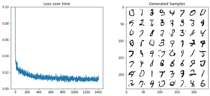

这看起来比我们的第一组结果好多了！您可以尝试调整 UNet 配置或更长时间的训练，以获得更好的性能。

损坏过程

DDPM 论文描述了一个为每个“timestep”添加少量噪声的损坏过程。为某些 timestep 给定 , 我们可以得到一个噪声稍稍增加的 :

这就是说，我们取 , 给他一个 的系数，然后加上带有 系数的噪声。这里 是根据一些管理器来为每一个 t 设定的，来决定每一个迭代周期中添加多少噪声。现在，我们不想把这个推演进行 500 次来得到 ，所以我们用另一个公式来根据给出的 计算得到任意 t 时刻的 :

数学符号看起来总是很吓人！幸运的是，调度器为我们处理了所有这些（取消下一个单元格的注释以检查代码）。我们可以画出 (标记为 sqrt_alpha_prod) 和 (标记为 sqrt_one_minus_alpha_prod) 来看一下输入 (x) 与噪声是如何在不同迭代周期中量化和叠加的 :

#??noise_scheduler.add_noise

noise_scheduler = DDPMScheduler(num_train_timesteps=1000)
plt.plot(noise_scheduler.alphas_cumprod.cpu() ** 0.5, label=r"${\sqrt{\bar{\alpha}_t}}$")
plt.plot((1 - noise_scheduler.alphas_cumprod.cpu()) ** 0.5, label=r"$\sqrt{(1 - \bar{\alpha}_t)}$")
plt.legend(fontsize="x-large");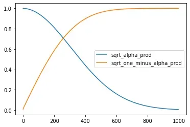

一开始 , 噪声 x 里绝大部分都是 x 自身的值  (sqrt_alpha_prod ~= 1)，但是随着时间的推移，x 的成分逐渐降低而噪声的成分逐渐增加。与我们根据 amount 对 x 和噪声进行线性混合不同，这个噪声的增加相对较快。我们可以在一些数据上看到这一点：

#@markdown visualize the DDPM noising process for different timesteps:

# Noise a batch of images to view the effect
fig, axs = plt.subplots(3, 1, figsize=(16, 10))
xb, yb = next(iter(train_dataloader))
xb = xb.to(device)[:8]
xb = xb * 2. - 1. # Map to (-1, 1)
print('X shape', xb.shape)

# Show clean inputs
axs[0].imshow(torchvision.utils.make_grid(xb[:8])[0].detach().cpu(), cmap='Greys')
axs[0].set_title('Clean X')

# Add noise with scheduler
timesteps = torch.linspace(0, 999, 8).long().to(device)
noise = torch.randn_like(xb) # << NB: randn not rand
noisy_xb = noise_scheduler.add_noise(xb, noise, timesteps)
print('Noisy X shape', noisy_xb.shape)

# Show noisy version (with and without clipping)
axs[1].imshow(torchvision.utils.make_grid(noisy_xb[:8])[0].detach().cpu().clip(-1, 1),  cmap='Greys')
axs[1].set_title('Noisy X (clipped to (-1, 1)')
axs[2].imshow(torchvision.utils.make_grid(noisy_xb[:8])[0].detach().cpu(),  cmap='Greys')
axs[2].set_title('Noisy X');

X shape torch.Size([8, 1, 28, 28])
Noisy X shape torch.Size([8, 1, 28, 28])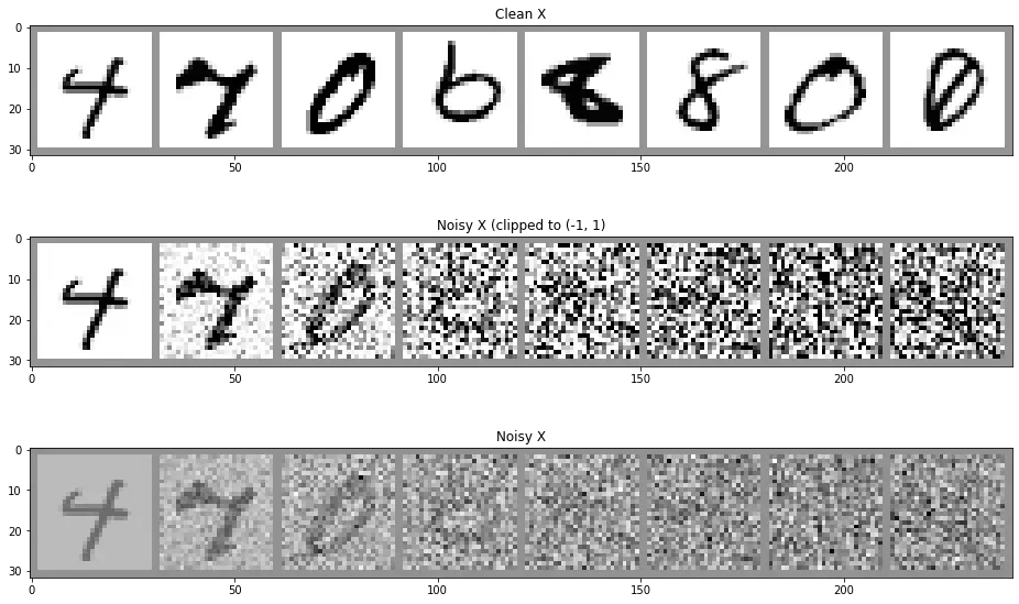

在运行中的另一个变化：在 DDPM 版本中，加入的噪声是取自一个高斯分布（来自均值 0 方差 1 的 torch.randn），而不是在我们原始 corrupt 函数中使用的 0-1 之间的均匀分布（torch.rand），当然对训练数据做正则化也可以理解。在另一篇笔记中，你会看到 Normalize(0.5, 0.5) 函数在变化列表中，它把图片数据从 (0, 1) 区间映射到 (-1, 1)，对我们的目标来说也‘足够用了’。我们在此篇笔记中没使用这个方法，但在上面的可视化中为了更好的展示添加了这种做法。

训练目标

在我们的玩具示例中，我们让模型尝试预测去噪图像。在 DDPM 和许多其他扩散模型实现中，模型则会预测损坏过程中使用的噪声（在缩放之前，因此是单位方差噪声）。在代码中，它看起来像是这样：

noise = torch.randn_like(xb) # << NB: randn not rand
noisy_x = noise_scheduler.add_noise(x, noise, timesteps)
model_prediction = model(noisy_x, timesteps).sample
loss = mse_loss(model_prediction, noise) # noise as the target

你可能认为预测噪声（我们可以从中得出去噪图像的样子）等同于直接预测去噪图像。那么，为什么要这么做呢？这仅仅是为了数学上的方便吗？

这里其实还有另一些精妙之处。我们在训练过程中，会计算不同（随机选择）timestep 的 loss。这些不同的目标将导致这些 loss 的不同的“隐含权重”，其中预测噪声会将更多的权重放在较低的噪声水平上。你可以选择更复杂的目标来改变这种“隐性损失权重”。或者，您选择的噪声管理器将在较高的噪声水平下产生更多的示例。也许你让模型设计成预测 “velocity” v，我们将其定义为由噪声水平影响的图像和噪声组合（请参阅“扩散模型快速采样的渐进蒸馏”- ‘PROGRESSIVE DISTILLATION FOR FAST SAMPLING OF DIFFUSION MODELS’）。也许你将模型设计成预测噪声，然后基于某些因子来对 loss 进行缩放：比如有些理论指出可以参考噪声水平（参见“扩散模型的感知优先训练”-‘Perception Prioritized Training of Diffusion Models’），或者基于一些探索模型最佳噪声水平的实验（参见“基于扩散的生成模型的设计空间说明”-‘Elucidating the Design Space of Diffusion-Based Generative Models’）。

一句话解释：选择目标对模型性能有影响，现在有许多研究者正在探索“最佳”选项是什么。目前，预测噪声（epsilon 或 eps）是最流行的方法，但随着时间的推移，我们很可能会看到库中支持的其他目标，并在不同的情况下使用。

迭代周期（Timestep）调节

UNet2DModel 以 x 和 timestep 为输入。后者被转化为一个嵌入（embedding），并在多个地方被输入到模型中。

这背后的理论支持是这样的：通过向模型提供有关噪声水平的信息，它可以更好地执行任务。虽然在没有这种 timestep 条件的情况下也可以训练模型，但在某些情况下，它似乎确实有助于性能，目前来说绝大多数的模型实现都包括了这一输入。

取样（采样）

有一个模型可以用来预测在带噪样本中的噪声（或者说能预测其去噪版本），我们怎么用它来生成图像呢？

我们可以给入纯噪声，然后就希望模型能一步就输出一个不带噪声的好图像。但是，就我们上面所见到的来看，这通常行不通。所以，我们在模型预测的基础上使用足够多的小步，迭代着来每次去除一点点噪声。

具体我们怎么走这些小步，取决于使用上面取样方法。我们不会去深入讨论太多的理论细节，但是一些顶层想法是这样：

• 每一步你想走多大？也就是说，你遵循什么样的“噪声计划（噪声管理）”？

• 你只使用模型当前步的预测结果来指导下一步的更新方向吗（像 DDPM，DDIM 或是其他的什么那样）？你是否要使用模型来多预测几次来估计一个更高阶的梯度来更新一步更大更准确的结果（更高阶的方法和一些离散 ODE 处理器）？或者保留历史预测值来尝试更好的指导当前步的更新（线性多步或遗传取样器）？

• 你是否会在取样过程中额外再加一些随机噪声，或你完全已知的（deterministic）来添加噪声？许多取样器通过参数（如 DDIM 中的 ‘eta’）来供用户选择。

对于扩散模型取样器的研究演进的很快，随之开发出了越来越多可以使用更少步就找到好结果的方法。勇敢和有好奇心的人可能会在浏览 diffusers library 中不同部署方法时感到非常有意思，可以查看 Schedulers 代码 或看看 Schedulers 文档，这里经常有一些相关的论文。

• Schedulers 代码:
  https://github.com/huggingface/diffusers/tree/main/src/diffusers/schedulers

• Schedulers 文档:
  https://huggingface.co/docs/diffusers/main/en/api/schedulers

结语

希望这可以从一些不同的角度来审视扩散模型提供一些帮助。这篇笔记是 Jonathan Whitaker 为 Hugging Face 课程所写的，如果你对从噪声和约束分类来生成样本的例子感兴趣。问题与 bug 可以通过 GitHub issues 或 Discord 来交流。

中文版扩散模型课程：第一单元 – 智源社区

扩散模型课程第一单元第二部分：扩散模型从零到一 – 智源社区