源码来自[https://blog.csdn.net/qq_34467412/article/details/90738232]，作者也是对论文作者ResNet框架的复现，而我是在chatGPT帮助下把博主TensorFlow的代码改成了pytorch代码。
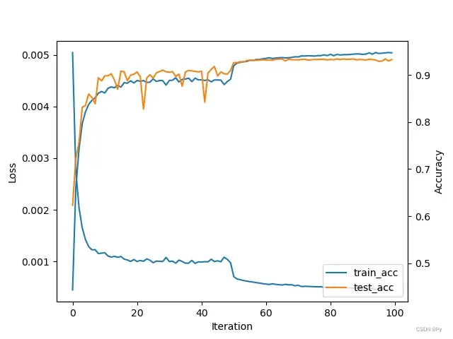
        由于硬件限制，并没有使用完整的数据集，仅对前10种调制模型进行识别，全信噪比情况下测试集识别率可达72%；仅考虑0：30dB情况下测试集识别率可达94%。

训练过程

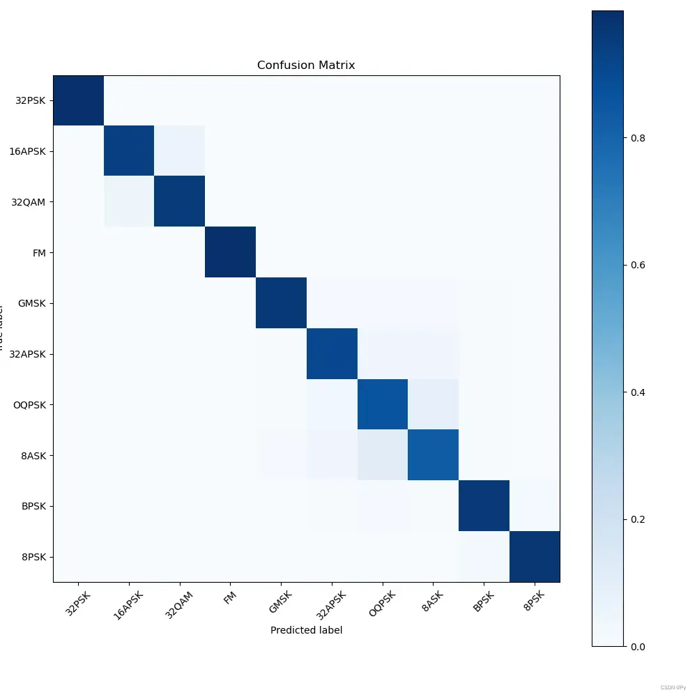
测试集上的混淆矩阵

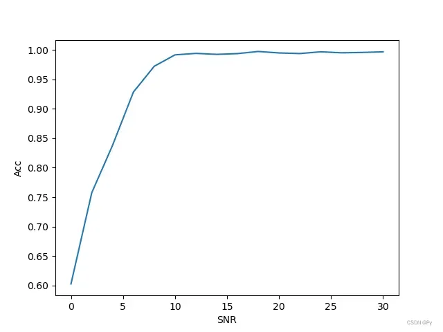
不同信噪比下的识别率

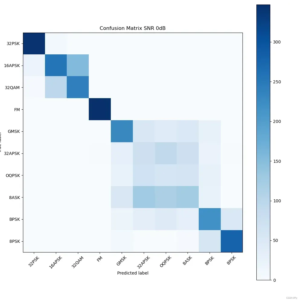
信噪比为0db时候的混淆矩阵

网络部分

class ResidualStack(nn.Module):
    def __init__(self, input_channels, output_channels, kernel_size, seq, pool_size):
        super(ResidualStack, self).__init__()
        self.conv1 = nn.Conv2d(input_channels, output_channels, kernel_size=1, stride=1, padding='same') # (kernel_size-1)//2保证输入输出形状一样
        # Residual Unit 1
        self.conv2 = nn.Conv2d(output_channels, 32, kernel_size=kernel_size, stride=1, padding='same')
        self.conv3 = nn.Conv2d(32, output_channels, kernel_size=kernel_size, stride=1, padding='same')
        # Residual Unit 2
        self.conv4 = nn.Conv2d(output_channels, 32, kernel_size=kernel_size, stride=1, padding='same')
        self.conv5 = nn.Conv2d(32, output_channels, kernel_size=kernel_size, stride=1, padding='same')
        self.maxpool = nn.MaxPool2d(kernel_size=pool_size, stride=pool_size)
        self.seq = seq

    def forward(self, x):
        # Residual Unit 1
        x = self.conv1(x)
        shortcut = x
        x = self.conv2(x)
        x = F.relu(x)
        x = self.conv3(x)
        x = x + shortcut
        x = F.relu(x)
        # Residual Unit 2
        shortcut = x
        x = self.conv4(x)
        x = F.relu(x)
        x = self.conv5(x)
        x = x + shortcut
        x = F.relu(x)
        x = self.maxpool(x)
        return x

class MyResNet(nn.Module):          # 1,1024,2
    def __init__(self, num_classes):
        super(MyResNet, self).__init__()
        self.num_classes = num_classes
        # self.bn = nn.BatchNorm2d(1)
        self.seq1 = ResidualStack(1, 32, kernel_size=(3, 2), seq="ReStk0", pool_size=(2, 2))
        self.seq2 = ResidualStack(32, 32, kernel_size=(3, 1), seq="ReStk1", pool_size=(2, 1))
        self.seq3 = ResidualStack(32, 32, kernel_size=(3, 1), seq="ReStk2", pool_size=(2, 1))
        self.seq4 = ResidualStack(32, 32, kernel_size=(3, 1), seq="ReStk3", pool_size=(2, 1))
        self.seq5 = ResidualStack(32, 32, kernel_size=(3, 1), seq="ReStk4", pool_size=(2, 1))
        self.seq6 = ResidualStack(32, 32, kernel_size=(3, 1), seq="ReStk5", pool_size=(2, 1))
        self.fc1 = nn.Linear(512, 128)           # 64 rml, 192 mnist, 512 rml2018
        self.fc2 = nn.Linear(128, num_classes)
        self.dropout = nn.AlphaDropout(0.2)

    def forward(self, x):
        # x = self.bn(x)
        x = self.seq1(x)
        x = self.seq2(x)
        x = self.seq3(x)
        x = self.seq4(x)
        x = self.seq5(x)
        x = self.seq6(x)
        x = torch.flatten(x,start_dim=1)
        x = self.fc1(x)
        x = F.selu(x)
        x = self.dropout(x)
        x = self.fc2(x)
        return x

 混淆矩阵代码

def plot_confusion_matrix(dataloader, model, classes):
    # pre-progression
    num_classes = len(classes)
    matrix = torch.zeros(size=(num_classes,num_classes))
    for x, y in dataloader:
        y_pred = model(x)
        for i in range(y.size(0)):
            matrix[y_pred[i].argmax()][y[i].argmax()] += 1
    for i in range(0, num_classes):
        matrix[i, :] = matrix[i, :] / torch.sum(matrix[i, :])
    # configuration of plot
    plt.figure(figsize=(10, 10))
    plt.imshow(matrix, interpolation='nearest', cmap=plt.cm.Blues)
    # interpolation插值影响图像显示效果
    tick_marks = np.arange(num_classes)
    plt.xticks(tick_marks, classes, rotation=45)
    plt.yticks(tick_marks, classes)
    plt.tight_layout()
    plt.title('Confusion Matrix')
    plt.colorbar()
    plt.xlabel('Predicted label')
    plt.ylabel('True label')
    plt.show()

    return matrix

 信噪比准确率，信噪比混淆矩阵代码

def plot_snr_curves(x, y, snr, model, classes):

    if not x[0].is_cuda:
        model.cpu()

    num_classes = len(classes)
    snr = snr.reshape((len(snr)))
    snrs, counts = np.unique(snr, return_counts=True)
    num_snrs = len(snrs)
    acc = np.zeros(num_snrs)
    matrix = torch.zeros(size=(num_snrs, num_classes, num_classes))
    for i in range(num_snrs):
        x_snr = x[snr==snrs[i]]
        y_snr = y[snr==snrs[i]]

        temp_dataset = Data.TensorDataset(x_snr, y_snr)
        temp_dataloader = DataLoader(dataset=temp_dataset, batch_size=256)

        for temp_x, temp_y in temp_dataloader:
            y_pred = model(temp_x)
            acc[i] += (y_pred.argmax(1) == temp_y.argmax(1)).sum()

            for k in range(temp_y.size(0)):
                matrix[i][y_pred[k].argmax()][temp_y[k].argmax()] += 1

    acc = acc / counts

    plt.plot(snrs, acc)
    plt.xlabel('SNR')
    plt.ylabel('Acc')
    plt.show()

    plt.figure(figsize=(10, 10))
    plt.imshow(matrix[0][:][:], interpolation='nearest', cmap=plt.cm.Blues)
    # interpolation插值影响图像显示效果
    tick_marks = np.arange(num_classes)
    plt.xticks(tick_marks, classes, rotation=45)
    plt.yticks(tick_marks, classes)
    plt.tight_layout()
    plt.title('Confusion Matrix SNR 0dB')
    plt.colorbar()
    plt.xlabel('Predicted label')
    plt.ylabel('True label')
    plt.show()
    return matrix

重新配置信号的label

def select(y, classes, classes_included=True):
    temp = y.sum(axis=0)
    one_zero = (temp >= 1)                              # 哪些地方是label的
    index = [i for i, x in enumerate(one_zero) if x]    # 得到label的位置
    new_classes = []
    new_num_classes = one_zero.sum()
    for i in range(new_num_classes):
        new_classes.append(classes[index[i]])

    new_y = np.zeros((y.shape[0], new_num_classes))
    y_index = y.argmax(1)                               # y=1的位置
    for i in range(y_index.shape[0]):
        new_y[i][y_index[i]] = 1

    if classes_included:
        return new_y, new_classes
    else:
        return new_y

训练和测试代码

def train(model, train_dataloader, itr, optimizer, loss_func):
    start_time = time.time()
    train_loss = 0
    train_accuracy = 0
    model.train()
    for x, y in train_dataloader:

        optimizer.zero_grad()       # 梯度清零
        y_pred = model(x)           # 计算预测标签
        loss = loss_func(y_pred, y.argmax(dim=1))  # 计算损失, argmax() for one-hot
        loss.backward()             # 利用反向传播计算gradients
        optimizer.step()            # 利用gradients更新参数值
        train_accuracy += (y_pred.argmax(1) == y.argmax(1)).sum()

        train_loss += loss.item()
    ep_loss = train_loss / len(train_dataloader.dataset)
    ep_train_acc = train_accuracy / len(train_dataloader.dataset)
    end_time = time.time()
    print("Epoch:", itr + 1,
          "\nTraining Loss: ", round(ep_loss,5),
          "Training Accuracy： ", round(ep_train_acc.item(), 5))
    print("Training time consuming: {}".format(end_time-start_time))
    return ep_loss, ep_train_acc

def test(model,test_dataloader):
    # test
    test_accuracy = 0
    model.eval()
    for x, y in test_dataloader:
        y_pred = model(x)
        test_accuracy += (y_pred.argmax(1) == y.argmax(1)).sum()

    ep_test_acc = test_accuracy / len(test_dataloader.dataset)
    print("Test Accuracy: ", round(ep_test_acc.item(),5))

    return ep_test_acc

主程序

if __name__ == "__main__":
    # Running Time
    time = datetime.datetime.now()
    month = time.month
    day = time.day

    # Configuration

    device = torch.device('cuda' if torch.cuda.is_available() else 'cpu')

    # File path
    path = 'data/SNR_greater_0_10data/'
    x_train, x_test, y_train, y_test = np.load(path + 'X_train.npy'), np.load(path + 'X_test.npy'), np.load(path + 'Y_train.npy'), np.load(path + 'Y_test.npy')
    y_train, classes = select(y_train, classes)
    y_test = select(y_test, classes, False)
    x_train, x_test, y_train, y_test = torch.from_numpy(x_train), torch.from_numpy(x_test), torch.from_numpy(y_train), torch.from_numpy(y_test)
    x_train, x_test, y_train, y_test = x_train.to(device), x_test.to(device), y_train.to(device), y_test.to(device)

    num_classes = len(classes)
    train_mean, train_std = torch.mean(x_train), torch.std(x_train)
    test_mean, test_std = torch.mean(x_test), torch.std(x_test)

    train_transformer = transforms.Compose([
        transforms.Normalize(mean=train_mean, std=train_std),
    ])
    test_transformer = transforms.Compose([
        transforms.Normalize(mean=test_mean, std=test_std),
    ])

    x_train = train_transformer(x_train)
    x_test = test_transformer(x_test)
    x_train = resize(x_train, (x_train.shape[0], 1, 1024, 2))
    x_test = resize(x_test, (x_test.shape[0], 1, 1024, 2))
    print("Shape of x_train : {}".format(x_train.shape))

    train_dataset = Data.TensorDataset(x_train, y_train)
    train_dataloader = DataLoader(dataset=train_dataset,batch_size=256, shuffle=True)
    test_dataset = Data.TensorDataset(x_test, y_test)
    test_dataloader = DataLoader(dataset=test_dataset, batch_size=256, shuffle=True)

    # Model
    model = MyResNet(num_classes).to(device)
    loss_function = nn.CrossEntropyLoss()
    optimizer = torch.optim.Adam(model.parameters(), lr=0.005)
    lr_scheduler = torch.optim.lr_scheduler.StepLR(optimizer, step_size=50, gamma=0.1)  # step decay

    itrs = 100
    train_loss = []
    train_acc = []
    test_acc = []
    best_accuracy = 0

    print("start training")
    for itr in range(itrs):
        epoch_loss, epoch_train_acc = train(model, train_dataloader, itr, optimizer, loss_function)
        epoch_test_acc = test(model, test_dataloader)
        train_loss.append(epoch_loss)
        train_acc.append(epoch_train_acc)
        test_acc.append(epoch_test_acc)

        # Save best model on test data
        if epoch_test_acc > best_accuracy:
            best_accuracy = epoch_test_acc
            torch.save(model, path + "ResNet_Identification_best_{}month_{}day.pth".format(month,day))
            print("-----The best accuracy now is {}-----".format(best_accuracy))
            print("-----The best model until now has been saved-----")
        lr_scheduler.step()

    confusion_matrix = plot_confusion_matrix(test_dataloader, model, classes)
    # Accuracy and Loss
    train_acc = [tensor.item() for tensor in train_acc]
    test_acc = [tensor.item() for tensor in test_acc]
    fig, ax1 = plt.subplots()
    ax2 = ax1.twinx()
    x = range(itrs)
    ax1.plot(x, train_loss, label='train_loss')
    ax2.plot(x, train_acc, label='train_acc')
    ax2.plot(x, test_acc, label='test_acc')

    ax1.set_xlabel('Iteration')
    ax1.set_ylabel('Loss')
    ax2.set_ylabel('Accuracy')
    plt.legend()
    plt.show()