密度峰值聚类算法DPC(Density Peak Clustering)理论基础与python实现

密度峰值聚类算法DPC(Density Peak Clustering)

基于密度峰值的聚类算法全称为基于快速搜索和发现密度峰值的聚类算法(clustering by fast search and find of density peaks, DPC)。它是2014年在Science上提出的聚类算法，该算法能够自动地发现簇中心，实现任意形状数据的高效聚类。

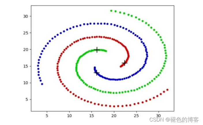
密度峰值聚类算法是对K-Means算法的一种改进，回顾K-Means算法，它需要人为指定聚类的簇的个数K，并且需要不断地去迭代更新聚类中心。如果K值指定的不恰当，那么最终得到的结果也将千差万别。此外K-Means算法在迭代过程中容易受到离群点的干扰，对于非簇状的数据效果很差。如下图的聚类结果，几乎不能使用K-Means算法得到。

密度峰值聚类（DP）算法是一种不需要迭代的，可以一次性找到聚类中心的方法聚类方法。（当时看到这篇文章的时候还是很震惊的，毕竟是发表在顶级刊物Science上的文章）

密度峰值聚类算法有两个基本的假设：

• 1）聚类中心的密度（Density）应当比较大。
• 2）聚类中心应当离比其密度更大的点较远

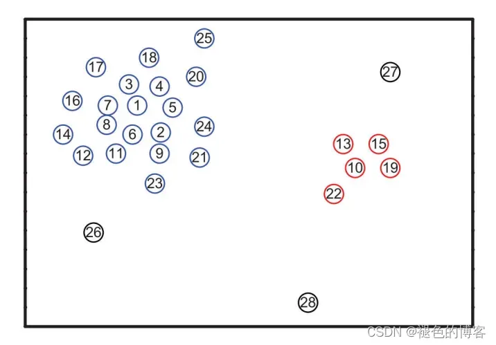
如上图所示：
点 1 密度最大是一个聚类中心；
点2,6,4密度也比较大，但是距离比他们密度更大的点（点1）太近，所以不是聚类中心；
点10 密度较大，且离密度比它大的点（1,2,4,6）较远是聚类中心；

基于以上两个假设，衍生出两个基本的概念：

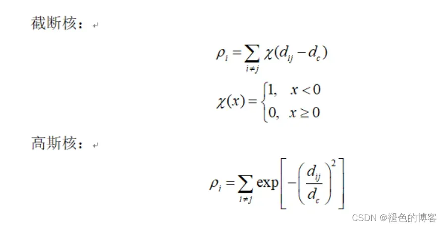
• 1）局部密度
  设有数据集为 ，其中 ，N为样本个数，M为样本维数。对于样本点i的局部密度，局部密度有两种计算方式，离散值采用截断核的计算方式，连续值则用高斯核的计算方式。
  

• 2)中心偏移距离
  相对距离 指样本点 i 与其他密度更高的点之间的最小距离。
  对于密度最高的样本，相对距离定义为：
  
  对于其余数据点，相对距离定义为：
  

密度峰值聚类算法认为两者都大的点就是聚类中心点

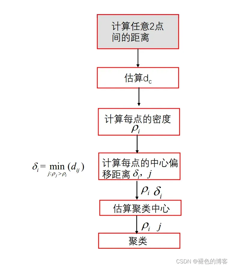
DPC算法的执行步骤

• 1）利用样本集数据计算距离矩阵；
• 2）确定邻域截断距离 ；
• 3）计算每个点的局部密度；
• 4）计算每个点的偏移距离，；
• 5）估算聚类中心点；
• 6）对非聚类中心数据点进行归类，聚类结束;
  最后可以将每个簇中的数据点进一步分为核心点和边缘点两个部分，并检测噪声点。其中，核心点是类簇核心部分，其 ρ ρρ 值较大；边缘点位于类簇的边界区域且 ρ ρρ 值较小，两者的区分界定则是借助于边界区域的平均局部密度。

密度峰值聚类算法DPC的python实现

导入需要用到的包

import numpy as np
import matplotlib.pyplot as plt

步骤一：计算数据点两两之间的距离

# 计算数据点两两之间的距离
def getDistanceMatrix(datas):
    N,D = np.shape(datas)
    dists = np.zeros([N,N])
    
    for i in range(N):
        for j in range(N):
            vi = datas[i,:]
            vj = datas[j,:]
            dists[i,j]= np.sqrt(np.dot((vi-vj),(vi-vj)))
    return dists

步骤二：确定邻域截断距离

# 找到密度计算的阈值dc
# 要求平均每个点周围距离小于dc的点的数目占总点数的1%-2%
def select_dc(dists):    
    '''算法1'''
    N = np.shape(dists)[0]
    tt = np.reshape(dists,N*N)
    percent = 2.0
    position = int(N * (N - 1) * percent / 100)
    dc = np.sort(tt)[position  + N]
    
    ''' 算法 2 '''
    # N = np.shape(dists)[0]
    # max_dis = np.max(dists)
    # min_dis = np.min(dists)
    # dc = (max_dis + min_dis) / 2
   
    # while True:
        # n_neighs = np.where(dists<dc)[0].shape[0]-N
        # rate = n_neighs/(N*(N-1))
        
        # if rate>=0.01 and rate<=0.02:
            # break
        # if rate<0.01:
            # min_dis = dc
        # else:
            # max_dis = dc
            
        # dc = (max_dis + min_dis) / 2
        # if max_dis - min_dis < 0.0001:
            # break
    return dc

步骤三：计算每个点的局部密度

# 计算每个点的局部密度    
def get_density(dists,dc,method=None):
    N = np.shape(dists)[0]
    rho = np.zeros(N)
    
    for i in range(N):
        if method == None:
            rho[i]  = np.where(dists[i,:]<dc)[0].shape[0]-1
        else:
            rho[i] = np.sum(np.exp(-(dists[i,:]/dc)**2))-1
    return rho

步骤四：计算每个点的偏移距离，

# 计算每个数据点的密度距离
# 即对每个点，找到密度比它大的所有点
# 再在这些点中找到距离其最近的点的距离
def get_deltas(dists,rho):
    N = np.shape(dists)[0]
    deltas = np.zeros(N)
    nearest_neiber = np.zeros(N)
    # 将密度从大到小排序
    index_rho = np.argsort(-rho)
    for i,index in enumerate(index_rho):
        # 对于密度最大的点
        if i==0:
            continue
            
        # 对于其他的点
        # 找到密度比其大的点的序号    
        index_higher_rho = index_rho[:i]
        # 获取这些点距离当前点的距离,并找最小值
        deltas[index] = np.min(dists[index,index_higher_rho])
        
        #保存最近邻点的编号
        index_nn = np.argmin(dists[index,index_higher_rho])
        nearest_neiber[index] = index_higher_rho[index_nn].astype(int)
    
    deltas[index_rho[0]] = np.max(deltas)   
    return deltas,nearest_neiber

步骤五：估算聚类中心点

# 通过阈值选取 rho与delta都大的点
# 作为聚类中心    
def find_centers_auto(rho,deltas):
    rho_threshold = (np.min(rho) + np.max(rho))/ 2
    delta_threshold  = (np.min(deltas) + np.max(deltas))/ 2
    N = np.shape(rho)[0]
    
    centers = []
    for i in range(N):
        if rho[i]>=rho_threshold and deltas[i]>delta_threshold:
            centers.append(i)
    return np.array(centers)

# 选取 rho与delta乘积较大的点作为
# 聚类中心   
def find_centers_K(rho,deltas,K):
    rho_delta = rho*deltas
    centers = np.argsort(-rho_delta)
    return centers[:K]

步骤六：对非聚类中心数据点进行归类

def cluster_PD(rho,centers,nearest_neiber):
    K = np.shape(centers)[0]
    if K == 0:
        print("can not find centers")
        return
    
    N = np.shape(rho)[0]
    labs = -1*np.ones(N).astype(int)
    
    # 首先对几个聚类中进行标号
    for i, center in enumerate(centers):
        labs[center] = i
   
    # 将密度从大到小排序
    index_rho = np.argsort(-rho)
    for i, index in enumerate(index_rho):
        # 从密度大的点进行标号
        if labs[index] == -1:
            # 如果没有被标记过
            # 那么聚类标号与距离其最近且密度比其大
            # 的点的标号相同
            labs[index] = labs[int(nearest_neiber[index])]
    return labs

可视化展示

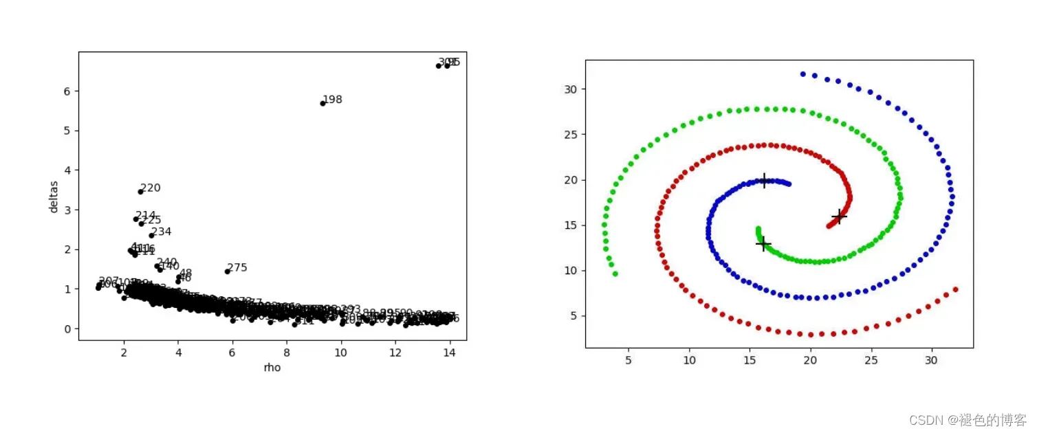
def draw_decision(rho,deltas,name="0_decision.jpg"):       
    plt.cla()
    for i in range(np.shape(datas)[0]):
        plt.scatter(rho[i],deltas[i],s=16.,color=(0,0,0))
        plt.annotate(str(i), xy = (rho[i], deltas[i]),xytext = (rho[i], deltas[i]))
        plt.xlabel("rho")
        plt.ylabel("deltas")
    plt.savefig(name)

def draw_cluster(datas,labs,centers, dic_colors, name="0_cluster.jpg"):     
    plt.cla()
    K = np.shape(centers)[0]
    
    for k in range(K):
        sub_index = np.where(labs == k)
        sub_datas = datas[sub_index]
        # 画数据点
        plt.scatter(sub_datas[:,0],sub_datas[:,1],s=16.,color=dic_colors[k])
        # 画聚类中心
        plt.scatter(datas[centers[k],0],datas[centers[k],1],color="k",marker="+",s = 200.)
    plt.savefig(name)

主函数入口

if __name__== "__main__":
    #画图保存的颜色卡
    dic_colors = {0:(.8,0,0),1:(0,.8,0),
                  2:(0,0,.8),3:(.8,.8,0),
                  4:(.8,0,.8),5:(0,.8,.8),
                  6:(0,0,0)}
    #读取文件
    file_name = "spiral"
    with open(file_name+".txt","r",encoding="utf-8") as f:
        lines = f.read().splitlines()
    lines = [line.split("\t")[:-1] for line in lines]
    datas = np.array(lines).astype(np.float32)    
    # 计算距离矩阵
    dists = getDistanceMatrix(datas)
    # 计算dc
    dc = select_dc(dists)
    print("dc",dc)
    # 计算局部密度 
    rho = get_density(dists,dc,method="Gaussion")
    # 计算密度距离
    deltas, nearest_neiber= get_deltas(dists,rho)  
    # 绘制密度/距离分布图
    draw_decision(rho,deltas,name=file_name+"_decision.jpg")
    # 获取聚类中心点
    centers = find_centers_K(rho,deltas,3)
    # centers = find_centers_auto(rho,deltas)
    print("centers",centers)
    #聚类
    labs = cluster_PD(rho,centers,nearest_neiber)
    #可视化展示
    draw_cluster(datas,labs,centers, dic_colors, name=file_name+"_cluster.jpg") 

结果展示如下：

31.95	7.95	3
31.15	7.3	3
30.45	6.65	3
29.7	6	3
28.9	5.55	3
28.05	5	3
27.2	4.55	3
26.35	4.15	3
25.4	3.85	3
24.6	3.6	3
23.6	3.3	3
22.75	3.15	3
21.85	3.05	3
20.9	3	3
20	2.9	3
19.1	3	3
18.2	3.2	3
17.3	3.25	3
16.55	3.5	3
15.7	3.7	3
14.85	4.1	3
14.15	4.4	3
13.4	4.75	3
12.7	5.2	3
12.05	5.65	3
11.45	6.15	3
10.9	6.65	3
10.3	7.25	3
9.7	7.85	3
9.35	8.35	3
8.9	9.05	3
8.55	9.65	3
8.15	10.35	3
7.95	10.95	3
7.75	11.7	3
7.55	12.35	3
7.45	13	3
7.35	13.75	3
7.3	14.35	3
7.35	14.95	3
7.35	15.75	3
7.55	16.35	3
7.7	16.95	3
7.8	17.55	3
8.05	18.15	3
8.3	18.75	3
8.65	19.3	3
8.9	19.85	3
9.3	20.3	3
9.65	20.8	3
10.2	21.25	3
10.6	21.65	3
11.1	22.15	3
11.55	22.45	3
11.95	22.7	3
12.55	23	3
13.05	23.2	3
13.45	23.4	3
14	23.55	3
14.55	23.6	3
15.1	23.75	3
15.7	23.75	3
16.15	23.85	3
16.7	23.8	3
17.15	23.75	3
17.75	23.75	3
18.2	23.6	3
18.65	23.5	3
19.1	23.35	3
19.6	23.15	3
20	22.95	3
20.4	22.7	3
20.7	22.55	3
21	22.15	3
21.45	21.95	3
21.75	21.55	3
22	21.25	3
22.25	21	3
22.5	20.7	3
22.65	20.35	3
22.75	20.05	3
22.9	19.65	3
23	19.35	3
23.1	19	3
23.15	18.65	3
23.2	18.25	3
23.2	18.05	3
23.2	17.8	3
23.1	17.45	3
23.05	17.15	3
22.9	16.9	3
22.85	16.6	3
22.7	16.4	3
22.6	16.2	3
22.55	16.05	3
22.4	15.95	3
22.35	15.8	3
22.2	15.65	3
22.15	15.55	3
22	15.4	3
21.9	15.3	3
21.85	15.25	3
21.75	15.15	3
21.65	15.05	3
21.55	15	3
21.5	14.9	3
19.35	31.65	1
20.35	31.45	1
21.35	31.1	1
22.25	30.9	1
23.2	30.45	1
23.95	30.05	1
24.9	29.65	1
25.6	29.05	1
26.35	28.5	1
27.15	27.9	1
27.75	27.35	1
28.3	26.6	1
28.95	25.85	1
29.5	25.15	1
29.95	24.45	1
30.4	23.7	1
30.6	22.9	1
30.9	22.1	1
31.25	21.3	1
31.35	20.55	1
31.5	19.7	1
31.55	18.9	1
31.65	18.15	1
31.6	17.35	1
31.45	16.55	1
31.3	15.8	1
31.15	15.05	1
30.9	14.35	1
30.6	13.65	1
30.3	13	1
29.9	12.3	1
29.5	11.75	1
29	11.15	1
28.5	10.6	1
28	10.1	1
27.55	9.65	1
26.9	9.1	1
26.25	8.8	1
25.7	8.4	1
25.15	8.05	1
24.5	7.75	1
23.9	7.65	1
23.15	7.4	1
22.5	7.3	1
21.9	7.1	1
21.25	7.05	1
20.5	7	1
19.9	6.95	1
19.25	7.05	1
18.75	7.1	1
18.05	7.25	1
17.5	7.35	1
16.9	7.6	1
16.35	7.8	1
15.8	8.05	1
15.4	8.35	1
14.9	8.7	1
14.45	8.9	1
13.95	9.3	1
13.6	9.65	1
13.25	10.1	1
12.95	10.55	1
12.65	10.9	1
12.35	11.4	1
12.2	11.75	1
11.95	12.2	1
11.8	12.65	1
11.75	13.05	1
11.55	13.6	1
11.55	14	1
11.55	14.35	1
11.55	14.7	1
11.6	15.25	1
11.65	15.7	1
11.8	16.05	1
11.85	16.5	1
12	16.75	1
12.15	17.2	1
12.3	17.6	1
12.55	17.85	1
12.8	18.05	1
13.1	18.4	1
13.3	18.6	1
13.55	18.85	1
13.8	19.05	1
14.15	19.25	1
14.45	19.5	1
14.85	19.55	1
15	19.7	1
15.25	19.7	1
15.55	19.85	1
15.95	19.9	1
16.2	19.9	1
16.55	19.9	1
16.85	19.9	1
17.2	19.9	1
17.4	19.8	1
17.65	19.75	1
17.8	19.7	1
18	19.6	1
18.2	19.55	1
3.9	9.6	2
3.55	10.65	2
3.35	11.4	2
3.1	12.35	2
3.1	13.25	2
3.05	14.15	2
3	15.1	2
3.1	16	2
3.2	16.85	2
3.45	17.75	2
3.7	18.7	2
3.95	19.55	2
4.35	20.25	2
4.7	21.1	2
5.15	21.8	2
5.6	22.5	2
6.2	23.3	2
6.8	23.85	2
7.35	24.45	2
8.05	24.95	2
8.8	25.45	2
9.5	26	2
10.2	26.35	2
10.9	26.75	2
11.7	27	2
12.45	27.25	2
13.3	27.6	2
14.05	27.6	2
14.7	27.75	2
15.55	27.75	2
16.4	27.75	2
17.1	27.75	2
17.9	27.75	2
18.55	27.7	2
19.35	27.6	2
20.1	27.35	2
20.7	27.1	2
21.45	26.8	2
22.05	26.5	2
22.7	26.15	2
23.35	25.65	2
23.8	25.3	2
24.3	24.85	2
24.75	24.35	2
25.25	23.95	2
25.65	23.45	2
26.05	23	2
26.2	22.3	2
26.6	21.8	2
26.75	21.25	2
27	20.7	2
27.15	20.15	2
27.15	19.6	2
27.35	19.1	2
27.35	18.45	2
27.4	18	2
27.3	17.4	2
27.15	16.9	2
27	16.4	2
27	15.9	2
26.75	15.35	2
26.55	14.85	2
26.3	14.45	2
25.95	14.1	2
25.75	13.7	2
25.35	13.3	2
25.05	12.95	2
24.8	12.7	2
24.4	12.45	2
24.05	12.2	2
23.55	11.85	2
23.2	11.65	2
22.75	11.4	2
22.3	11.3	2
21.9	11.1	2
21.45	11.05	2
21.1	11	2
20.7	10.95	2
20.35	10.95	2
19.95	11	2
19.55	11	2
19.15	11.05	2
18.85	11.1	2
18.45	11.25	2
18.15	11.35	2
17.85	11.5	2
17.5	11.7	2
17.2	11.95	2
17	12.05	2
16.75	12.2	2
16.65	12.35	2
16.5	12.5	2
16.35	12.7	2
16.2	12.8	2
16.15	12.95	2
16	13.1	2
15.95	13.25	2
15.9	13.4	2
15.8	13.5	2
15.8	13.65	2
15.75	13.85	2
15.65	14.05	2
15.65	14.25	2
15.65	14.5	2
15.65	14.6	2