[Python] 机器学习 – 常用数据集(Dataset)之糖尿病(diabetes)数据集介绍，数据可视化和使用案例

糖尿病(diabetes)数据集介绍

diabetes 是一个关于糖尿病的数据集， 该数据集包括442个病人的生理数据及一年以后的病情发展情况。

该数据集共442条信息，特征值总共10项, 如下:

age: 年龄

sex: 性别

bmi(body mass index): 身体质量指数，是衡量是否肥胖和标准体重的重要指标，理想BMI(18.5~23.9) = 体重(单位Kg) ÷ 身高的平方 (单位m)

bp(blood pressure): 血压（平均血压）

s1,s2,s3,s4,s4,s6: 六种血清的化验数据，是血液中各种疾病级数指针的6的属性值。

s1——tc，T细胞（一种白细胞）

s2——ldl，低密度脂蛋白

s3——hdl，高密度脂蛋白

s4——tch，促甲状腺激素

s5——ltg，拉莫三嗪

s6——glu，血糖水平

.. _diabetes_dataset:

Diabetes dataset
----------------

Ten baseline variables, age, sex, body mass index, average blood
pressure, and six blood serum measurements were obtained for each of n =
442 diabetes patients, as well as the response of interest, a
quantitative measure of disease progression one year after baseline.

**Data Set Characteristics:**

  :Number of Instances: 442

  :Number of Attributes: First 10 columns are numeric predictive values

  :Target: Column 11 is a quantitative measure of disease progression one year after baseline

  :Attribute Information:
      - age     age in years
      - sex
      - bmi     body mass index
      - bp      average blood pressure
      - s1      tc, total serum cholesterol
      - s2      ldl, low-density lipoproteins
      - s3      hdl, high-density lipoproteins
      - s4      tch, total cholesterol / HDL
      - s5      ltg, possibly log of serum triglycerides level
      - s6      glu, blood sugar level

Note: Each of these 10 feature variables have been mean centered and scaled by the standard deviation times the square root of `n_samples` (i.e. the sum of squares of each column totals 1).

Source URL:
Diabetes Data

For more information see:
Bradley Efron, Trevor Hastie, Iain Johnstone and Robert Tibshirani (2004) "Least Angle Regression," Annals of Statistics (with discussion), 407-499.
(https://web.stanford.edu/~hastie/Papers/LARS/LeastAngle_2002.pdf) 

加载糖尿病数据集diabetes并查看数据

sklearn.datasets.load_diabetes — scikit-learn 1.4.0 documentation

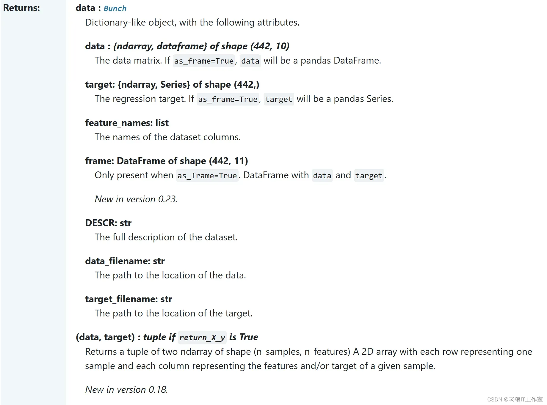
from sklearn.datasets import load_diabetes

diabete_datas = load_diabetes()

diabete_datas.data[0:5]

diabete_datas.data.shape

diabete_datas.target[0:5]

diabete_datas.target.shape

diabete_datas.feature_names

基于线性回归对数据集进行分析

Linear Regression Example — scikit-learn 1.4.0 documentation

import matplotlib.pyplot as plt
import numpy as np

from sklearn import datasets, linear_model
from sklearn.metrics import mean_squared_error, r2_score

# Load the diabetes dataset
diabetes_X, diabetes_y = datasets.load_diabetes(return_X_y=True)
print('diabetes_X:\n', diabetes_X[0:5])
print('diabetes_y:\n', diabetes_y[0:5])
# Use only one feature (bmi)
diabetes_X = diabetes_X[:, np.newaxis, 2]
print('diabetes_X:\n', diabetes_X[0:5])

# Split the data into training/testing sets
diabetes_X_train = diabetes_X[:-20]
diabetes_X_test = diabetes_X[-20:]

# Split the targets into training/testing sets
diabetes_y_train = diabetes_y[:-20]
diabetes_y_test = diabetes_y[-20:]

# Create linear regression object
regr = linear_model.LinearRegression()

# Train the model using the training sets
regr.fit(diabetes_X_train, diabetes_y_train)

# Make predictions using the testing set
diabetes_y_pred = regr.predict(diabetes_X_test)

# The coefficients
print("斜率 Coefficients: \n", regr.coef_)
# The intercept
print("截距(intercept): \n", regr.intercept_)
# The mean squared error
print("均方误差 Mean squared error: %.2f" % mean_squared_error(diabetes_y_test, diabetes_y_pred))
# The coefficient of determination: 1 is perfect prediction
print("R2分数(Coefficient of determination): %.2f" % r2_score(diabetes_y_test, diabetes_y_pred))

# Plot outputs
plt.scatter(diabetes_X_test, diabetes_y_test, color="black")
plt.plot(diabetes_X_test, diabetes_y_pred, color="blue", linewidth=3)


plt.show()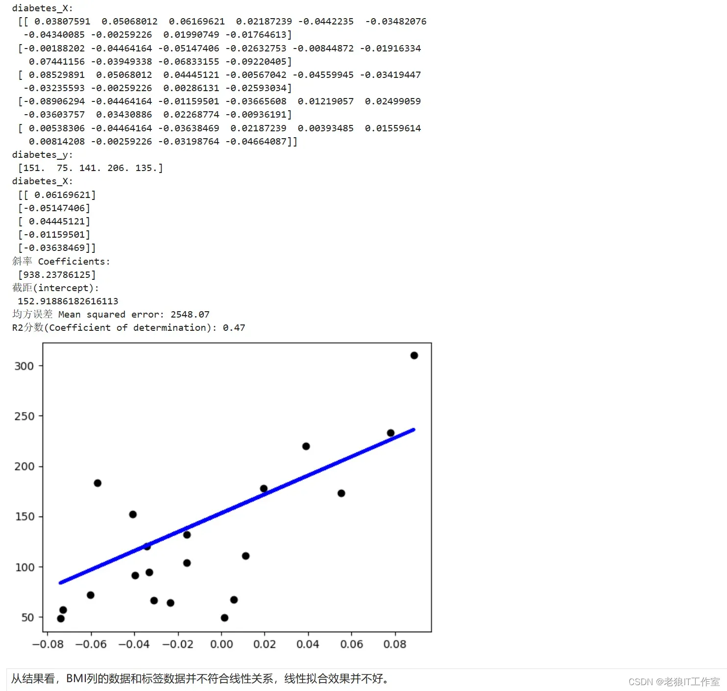

使用岭回归交叉验证找出最重要的特征

sklearn.linear_model.RidgeCV — scikit-learn 1.4.0 documentation

Model-based and sequential feature selection — scikit-learn 1.4.0 documentation

To get an idea of the importance of the features, we are going to use the RidgeCV estimator. The features with thehighest absolutecoef_value are considered the most important.We can observe the coefficients directly without needing to scale them (orscale the data) because from the description above, we know that the features were already standardized.

为了了解特征的重要性，我们将使用RidgeCV估计器。具有最高绝对有效值的特征被认为是最重要的。我们可以直接观察系数，而无需缩放它们（或缩放数据），因为从上面的描述中，我们知道特征值已经被标准化了。

import matplotlib.pyplot as plt
import numpy as np
from sklearn.linear_model import RidgeCV
from sklearn.datasets import load_diabetes

diabetes = load_diabetes()
X, y = diabetes.data, diabetes.target

ridge = RidgeCV(alphas=np.logspace(-6, 6, num=5)).fit(X, y)
importance = np.abs(ridge.coef_)
feature_names = np.array(diabetes.feature_names)
plt.bar(height=importance, x=feature_names)
plt.title("Feature importances via coefficients")
plt.show()

从上图可以看出，特征s1和s5的重要程度最高，特征bmi次之。