本文主要对人工势场法路径规划算法进行介绍,主要涉及人工势场法的简介、引力和斥力模型及其推导过程、人工势场法的缺陷及改进思路、人工势场法的Python与MATLAB开源源码等方面
一、人工势场法简介
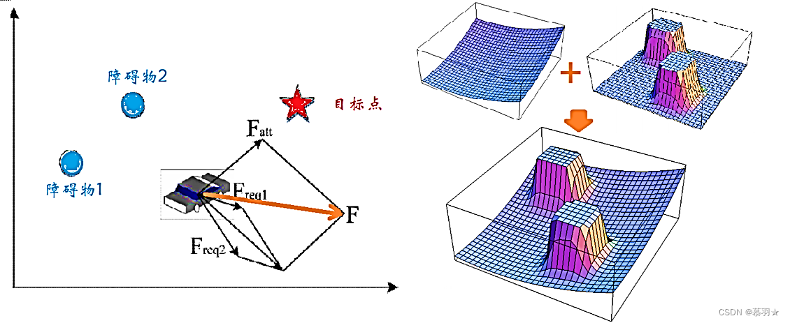
人工势场法是由Khatib于1985年在论文《Real-Time Obstacle Avoidance for Manipulators and Mobile Robots》中提出的一种虚拟力法。它的基本思想是将机器人在周围环境中的运动,设计成一种抽象的人造引力场中的运动,目标点对移动机器人产生“引力”,障碍物对移动机器人产生“斥力”,最后通过求合力来控制移动机器人的运动。应用势场法规划出来的路径一般是比较平滑并且安全,但是这种方法存在局部最优点问题。

二、引力与斥力模型及公式推导
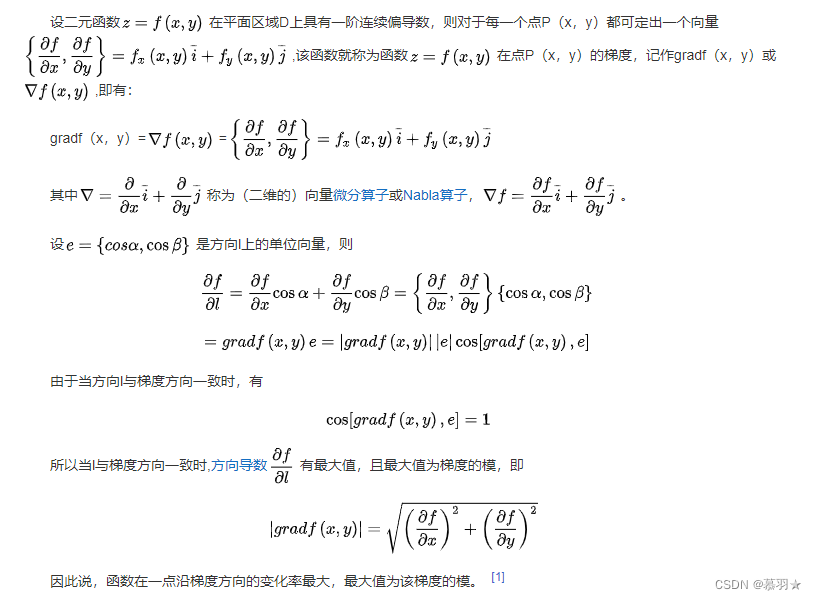
1、基础知识补充:梯度
梯度的本意是一个向量(矢量),表示某一函数在该点处的方向导数沿着该方向取得最大值,即函数在该点处沿着该方向(此梯度的方向)变化最快,变化率最大(为该梯度的模)。
2、引力与斥力模型
引力势场主要与机器人和目标点间的距离有关,距离越大,机器人所受的势能值就越大;距离越小,机器人所受的势能值则越小,所以引力势场的函数为:
其中η为正比例增益系数,ρ(q,qg)为一个矢量,表示机器人的位置q和目标点位置qg之间的欧几里德距离|q-qg|。矢量方向是从机器人的位置指向目标点位
置。
相应的引力为引力场的负梯度:
决定障碍物斥力势场的因素是机器人与障碍物间的距离,当机器人未进入障碍物的影响范围时,其受到的势能值为零;在机器人进入障碍物的影响范围后,两者之间的距离越大,机器人受到的斥力就越小,距离越小,机器人受到的斥力就越大,斥力势场的势场函数为:
其中k为正比例系数,ρ(q,qo)为一矢量,方向为从障碍物指向机器人,大小为机器人与障碍物间的距离|q-qo|,ρo为一常数,表示障碍物对机器人产生作用的最大距离。相应的斥力为斥力场的负梯度:
其中表示从
指向q的单位向量
3、引力与斥力公式的推导过程
设机器人位置为(x, y),障碍物位置为(xg, yg),则引力势场函数可由下式
改写为:
所以根据梯度下降法。在这种情况下,势场U的负梯度可被认为是位形空间中作用在机器人上的一个广义力,
斥力势场函数可由下式:
改写为:
所以:
其中对x求偏导部分过程如下:
同理,可得对y求偏导部分结果如下:
所以,斥力函数为:
三、算法缺陷
1、不能到达目标点的问题
当存在某个障碍物与目标点距离太近时,机器人到达目标点时,根据势场函数可知,目标点的引力降为零,而障碍物的斥力不为零,此时机器人虽到达目标点,但在斥力场的作用下不能停下来,从而导致目标点不可达的问题,机器人容易出现在目标点附近震荡的现象。
2、陷入局部最优的问题
机器人在某个位置时,如果若干个障碍物的合斥力与目标点的引力大小相等、方向相反,则合力为0,这将导致机器人受力为0,而停止运动,故无法继续向目标点移动,下图列举了其中的一种情况。

3、可能碰撞障碍物的问题
当物体离目标点比较远时,引力将变的特别大,相对较小的斥力在可以忽略的情况下,物体路径上可能会碰到障碍物
四、改进思路
1、优化斥力场函数
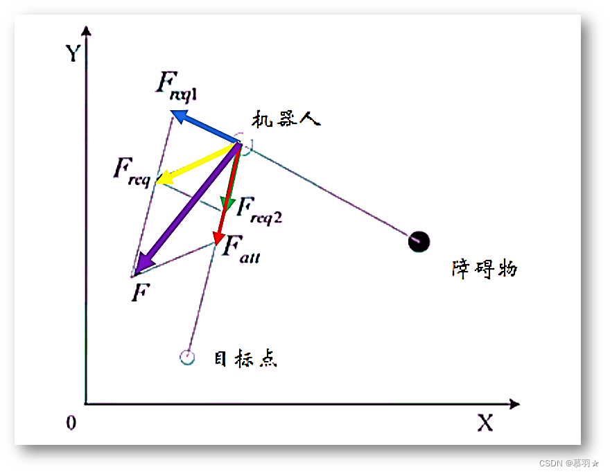
以上缺陷1和2的一种改进思路是,改变斥力场函数,传统的斥力场函数的大小由机器人与障碍物直接的距离决定,方向由障碍物指向机器人,为避免以上缺陷,我们可以把斥力场函数改为由两部分组成,第一部分像传统的斥力场函数一样由障碍物指向机器人,大小由机器人与障碍物之间距离和机器人与目标点距离共同决定,如下图中的蓝色箭头Freq1所示,第二部分斥力由机器人指向目标点,大小由机器人与障碍物之间距离和机器人与目标点之间距离共同决定,如下图中的绿色箭头Freq2所示,这两部分斥力共同组成了合斥力Freq,如下图中黄色箭头所示,再与红色箭头所示的引力Fatt求合力,得到最终机器人的受力,如紫色的箭头F所示。
上述改进思想的斥力函数如下,其中n为任意常数:
上述改进后,当机器人到达目标点时斥力也变为了0
2、针对陷入局部最小值问题的改进思路
针对陷入局部极小值问题,可以引入随机的虚拟力使机器人跳出局部极小值的状态。在障碍物密集的情况下,机器人易陷入局部最小值,此时,也可以对密集的障碍物进行处理,将多个障碍物看出一个整体来求斥力。此外,也可以通过设置子目标点的方式来使机器人逃出极小值。
五、开源程序
1、来自 白菜丁 的Python版本程序
(1)程序来源:局部路径规划-人工势场法【点击可跳转】
(2)程序如下所示:
import numpy as np
import matplotlib.pyplot as plt

# 初始化车的参数
d = 3.5  # 道路标准宽度
W = 1.8  # 汽车宽度
P0 = np.array([0, -d / 2, 1, 1])  # 车辆起点位置,分别代表x,y,vx,vy
Pg = np.array([99, d / 2, 0, 0])  # 目标点位置
Pobs = np.array([[15, 7 / 4, 0, 0],  # 障碍物位置
                 [30, -3 / 2, 0, 0],
                 [45, 3 / 2, 0, 0],
                 [60, -3 / 4, 0, 0],
                 [80, 7 / 4, 0, 0]])
P = np.array([[15, 7 / 4, 0, 0],
              [30, -3 / 2, 0, 0],
              [45, 3 / 2, 0, 0],
              [60, -3 / 4, 0, 0],
              [80, 7 / 4, 0, 0],
              [99, d / 2, 0, 0]])

Eta_att = 5  # 计算引力的增益系数
Eta_rep_ob = 15  # 计算斥力的增益系数
Eta_rep_edge = 50  # 计算边界斥力的增益系数

d0 = 20  # 障碍影响距离
n = len(P)  # 障碍物和目标总计个数
len_step = 0.5  # 步长
Num_iter = 200  # 最大循环迭代次数

Pi = P0
Path = []  # 存储路径
delta = np.zeros((n, 2))  # 存储每一个障碍到车辆的斥力方向向量以及引力方向向量
dist = []  # 存储每一个障碍到车辆的距离以及目标点到车辆距离
unitvector = np.zeros((n, 2))  # 存储每一个障碍到车辆的斥力单位向量以及引力单位向量
F_rep_ob = np.zeros((n - 1, 2))  # 存储每一个障碍到车辆的斥力
F_rep_edge = np.zeros((1, 2))
while ((Pi[0] - Pg[0]) ** 2 + (Pi[1] - Pg[1]) ** 2) ** 0.5 > 1:
    # a = ((Pi[0] - Pg[0]) ** 2 + (Pi[1] - Pg[1]) ** 2) ** 0.5
    Path.append(Pi.tolist())
    # 计算车辆当前位置和障碍物的单位方向向量
    for j in range(len(Pobs)):
        delta[j, :] = Pi[0:2] - P[j, 0:2]
        dist.append(np.linalg.norm(delta[j, :]))
        unitvector[j, :] = [delta[j, 0] / dist[j], delta[j, 1] / dist[j]]
    # 计算车辆当前位置和目标点的单位方向向量
    delta[n - 1, :] = P[n - 1, 0:2] - Pi[0:2]
    dist.append(np.linalg.norm(delta[n - 1, :]))
    unitvector[n - 1, :] = [delta[n - 1, 0] / dist[n - 1], delta[n - 1, 1] / dist[n - 1]]

    # 计算斥力
    for j in range(len(Pobs)):
        if dist[j] >= d0:
            F_rep_ob[j, :] = [0, 0]
        else:
            # 障碍物的斥力1,方向由障碍物指向车辆
            F_rep_ob1_abs = Eta_rep_ob * (1 / dist[j] - 1 / d0) * dist[n - 1] / dist[j] ** 2  # 回看公式设定n=1
            F_rep_ob1 = np.array([F_rep_ob1_abs * unitvector[j, 0], F_rep_ob1_abs * unitvector[j, 1]])
            # 障碍物的斥力2,方向由车辆指向目标点
            F_rep_ob2_abs = 0.5 * Eta_rep_ob * (1 / dist[j] - 1 / d0) ** 2
            F_rep_ob2 = np.array([F_rep_ob2_abs * unitvector[n - 1, 0], F_rep_ob2_abs * unitvector[n - 1, 1]])
            # 改进后的障碍物和斥力计算
            F_rep_ob[j, :] = F_rep_ob1 + F_rep_ob2
    # 增加的边界斥力
    if -d + W / 2 < Pi[1] <= -d / 2:
        # 这个边界斥力只作用在y方向,因此x方向为0
        F_rep_edge = [0, Eta_rep_edge * np.linalg.norm(Pi[2:4]) * np.exp(-d / 2 - Pi[1])]
    elif -d / 2 < Pi[1] <= -W / 2:
        F_rep_edge = [0, 1 / 3 * Eta_rep_edge * Pi[1] ** 2]
    elif W / 2 < Pi[1] <= d / 2:
        F_rep_edge = [0, -1 / 3 * Eta_rep_edge * Pi[1] ** 2]
    elif d / 2 < Pi[1] <= d - W / 2:
        F_rep_edge = [0, Eta_rep_edge * np.linalg.norm(Pi[2:4]) * np.exp(Pi[1] - d / 2)]

    # 计算合力和方向
    F_rep = [np.sum(F_rep_ob[:, 0]) + F_rep_edge[0], np.sum(F_rep_ob[:, 1]) + F_rep_edge[1]]  # 合并边界斥力和障碍舞斥力
    F_att = [Eta_att * dist[n - 1] * unitvector[n - 1, 0], Eta_att * dist[n - 1] * unitvector[n - 1, 1]]  # 引力向量
    F_sum = np.array([F_rep[0] + F_att[0], F_rep[1] + F_att[1]])
    UnitVec_Fsum = 1 / np.linalg.norm(F_sum) * F_sum
    # 计算车的下一步位置
    Pi[0:2] = Pi[0:2] + len_step * UnitVec_Fsum
# 将目标添加到路径中
Path.append(Pg.tolist())

# 画图
x = []  # 路径的x坐标
y = []  # 路径的y坐标
for val in Path:
    x.append(val[0])
    y.append(val[1])

plt.plot(x, y, linewidth=0.6)
plt.axhline(y=0, color='g', linestyle=':',linewidth=0.3)
plt.axis([-5,100,-4,4])
plt.gca().set_aspect('equal')
plt.plot(0, -d / 2, 'ro', markersize=1)
plt.plot(15, 7 / 4, 'ro', markersize=1)
plt.plot(30, -3 / 2, 'ro', markersize=1)
plt.plot(45, 3 / 2, 'ro', markersize=1)
plt.plot(60, -3 / 4, 'ro', markersize=1)
plt.plot(80, 7 / 4, 'ro', markersize=1)
plt.plot(99, d / 2, 'ro', markersize=1)
plt.xlabel('x')
plt.ylabel('y')
plt.show()
(3)程序分析:
首先是程序的初始化部分,对道路宽度、汽车宽度、起点和目标点位置、障碍物的位置、引力的增益系数、斥力的增益系数、边界增益系数、障碍物的影响距离、步长、最大循环次数(程序中未用到)等参数进行设定。
进入循环,只要机器人当前位置与目标点之间的距离大于1就循环执行以下程序,将机器人当前状态(位置和速度)(也可以是模拟的当前位置和速度)添加到路径中,然后计算机器人当前位置与障碍物和目标点之间的单位方向向量,然后计算斥力和引力的大小、计算边界带来的斥力,计算合力的大小和方向,更新机器人的状态(位置和速度),以此循环。
当机器人当前位置与目标点之间的距离小于1时,循环结束,绘制路径,程序结束。
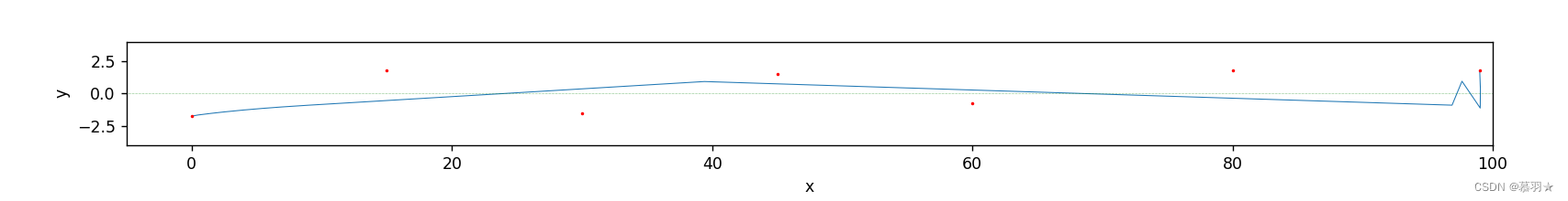
(4)上述程序运行结果示例:
2、来自 AtsushiSakai 的Python版本程序
(1)程序来源(GitHub链接):potential_field_planning.py【点击可跳转】
(2)程序如下所示:
""" Potential Field based path planner author: Atsushi Sakai (@Atsushi_twi) Ref: https://www.cs.cmu.edu/~motionplanning/lecture/Chap4-Potential-Field_howie.pdf """

from collections import deque
import numpy as np
import matplotlib.pyplot as plt

# Parameters
KP = 5.0  # attractive potential gain
ETA = 100.0  # repulsive potential gain
AREA_WIDTH = 30.0  # potential area width [m]
# the number of previous positions used to check oscillations
OSCILLATIONS_DETECTION_LENGTH = 3

show_animation = True


def calc_potential_field(gx, gy, ox, oy, reso, rr, sx, sy):
    """ 计算势场图 gx,gy: 目标坐标 ox,oy: 障碍物坐标列表 reso: 势场图分辨率 rr: 机器人半径 sx,sy: 起点坐标 """
    # 确定势场图坐标范围:
    minx = min(min(ox), sx, gx) - AREA_WIDTH / 2.0
    miny = min(min(oy), sy, gy) - AREA_WIDTH / 2.0
    maxx = max(max(ox), sx, gx) + AREA_WIDTH / 2.0
    maxy = max(max(oy), sy, gy) + AREA_WIDTH / 2.0
    # 根据范围和分辨率确定格数:
    xw = int(round((maxx - minx) / reso))
    yw = int(round((maxy - miny) / reso))

    # calc each potential
    pmap = [[0.0 for i in range(yw)] for i in range(xw)]

    for ix in range(xw):
        x = ix * reso + minx   # 根据索引和分辨率确定x坐标

        for iy in range(yw):
            y = iy * reso + miny  # 根据索引和分辨率确定x坐标
            ug = calc_attractive_potential(x, y, gx, gy)  # 计算引力
            uo = calc_repulsive_potential(x, y, ox, oy, rr)  # 计算斥力
            uf = ug + uo
            pmap[ix][iy] = uf

    return pmap, minx, miny


def calc_attractive_potential(x, y, gx, gy):
    """ 计算引力势能:1/2*KP*d """
    return 0.5 * KP * np.hypot(x - gx, y - gy)


def calc_repulsive_potential(x, y, ox, oy, rr):
    """ 计算斥力势能: 如果与最近障碍物的距离dq在机器人膨胀半径rr之内:1/2*ETA*(1/dq-1/rr)**2 否则:0.0 """
    # search nearest obstacle
    minid = -1
    dmin = float("inf")
    for i, _ in enumerate(ox):
        d = np.hypot(x - ox[i], y - oy[i])
        if dmin >= d:
            dmin = d
            minid = i

    # calc repulsive potential
    dq = np.hypot(x - ox[minid], y - oy[minid])

    if dq <= rr:
        if dq <= 0.1:
            dq = 0.1

        return 0.5 * ETA * (1.0 / dq - 1.0 / rr) ** 2
    else:
        return 0.0


def get_motion_model():
    # dx, dy
    # 九宫格中 8个可能的运动方向
    motion = [[1, 0],
              [0, 1],
              [-1, 0],
              [0, -1],
              [-1, -1],
              [-1, 1],
              [1, -1],
              [1, 1]]

    return motion


def oscillations_detection(previous_ids, ix, iy):
    """ 振荡检测:避免“反复横跳” """
    previous_ids.append((ix, iy))

    if (len(previous_ids) > OSCILLATIONS_DETECTION_LENGTH):
        previous_ids.popleft()

    # check if contains any duplicates by copying into a set
    previous_ids_set = set()
    for index in previous_ids:
        if index in previous_ids_set:
            return True
        else:
            previous_ids_set.add(index)
    return False


def potential_field_planning(sx, sy, gx, gy, ox, oy, reso, rr):

    # calc potential field
    pmap, minx, miny = calc_potential_field(gx, gy, ox, oy, reso, rr, sx, sy)

    # search path
    d = np.hypot(sx - gx, sy - gy)
    ix = round((sx - minx) / reso)
    iy = round((sy - miny) / reso)
    gix = round((gx - minx) / reso)
    giy = round((gy - miny) / reso)

    if show_animation:
        draw_heatmap(pmap)
        # for stopping simulation with the esc key.
        plt.gcf().canvas.mpl_connect('key_release_event',
                lambda event: [exit(0) if event.key == 'escape' else None])
        plt.plot(ix, iy, "*k")
        plt.plot(gix, giy, "*m")

    rx, ry = [sx], [sy]
    motion = get_motion_model()
    previous_ids = deque()

    while d >= reso:
        minp = float("inf")
        minix, miniy = -1, -1
        # 寻找8个运动方向中势场最小的方向
        for i, _ in enumerate(motion):
            inx = int(ix + motion[i][0])
            iny = int(iy + motion[i][1])
            if inx >= len(pmap) or iny >= len(pmap[0]) or inx < 0 or iny < 0:
                p = float("inf")  # outside area
                print("outside potential!")
            else:
                p = pmap[inx][iny]
            if minp > p:
                minp = p
                minix = inx
                miniy = iny
        ix = minix
        iy = miniy
        xp = ix * reso + minx
        yp = iy * reso + miny
        d = np.hypot(gx - xp, gy - yp)
        rx.append(xp)
        ry.append(yp)
        # 振荡检测,以避免陷入局部最小值:
        if (oscillations_detection(previous_ids, ix, iy)):
            print("Oscillation detected at ({},{})!".format(ix, iy))
            break

        if show_animation:
            plt.plot(ix, iy, ".r")
            plt.pause(0.01)

    print("Goal!!")

    return rx, ry


def draw_heatmap(data):
    data = np.array(data).T
    plt.pcolor(data, vmax=100.0, cmap=plt.cm.Blues)


def main():
    print("potential_field_planning start")

    sx = 0.0  # start x position [m]
    sy = 10.0  # start y positon [m]
    gx = 30.0  # goal x position [m]
    gy = 30.0  # goal y position [m]
    grid_size = 0.5  # potential grid size [m]
    robot_radius = 5.0  # robot radius [m]
    # 以下障碍物坐标是我进行修改后的,用来展示人工势场法的困于局部最优的情况:
    ox = [15.0, 5.0, 20.0, 25.0, 12.0, 15.0, 19.0, 28.0, 27.0, 23.0, 30.0, 32.0]  # obstacle x position list [m]
    oy = [25.0, 15.0, 26.0, 25.0, 12.0, 20.0, 29.0, 28.0, 26.0, 25.0, 28.0, 27.0]  # obstacle y position list [m]

    if show_animation:
        plt.grid(True)
        plt.axis("equal")

    # path generation
    _, _ = potential_field_planning(
        sx, sy, gx, gy, ox, oy, grid_size, robot_radius)

    if show_animation:
        plt.show()


if __name__ == '__main__':
    print(__file__ + " start!!")
    main()
    print(__file__ + " Done!!")
(3)上述程序运行结果示例:

3、来自 ShuiXinYun的Python版本程序
(1)程序来源(GitHub链接):Artificial_Potential_Field【点击可跳转】
(2)程序Original_APF.py如下所示:
"""
人工势场寻路算法实现
最基本的人工势场,存在目标点不可达及局部最小点问题
"""
import math
import random
from matplotlib import pyplot as plt
from matplotlib.patches import Circle
import time


class Vector2d():
    """
    2维向量, 支持加减, 支持常量乘法(右乘)
    """

    def __init__(self, x, y):
        self.deltaX = x
        self.deltaY = y
        self.length = -1
        self.direction = [0, 0]
        self.vector2d_share()

    def vector2d_share(self):
        if type(self.deltaX) == type(list()) and type(self.deltaY) == type(list()):
            deltaX, deltaY = self.deltaX, self.deltaY
            self.deltaX = deltaY[0] - deltaX[0]
            self.deltaY = deltaY[1] - deltaX[1]
            self.length = math.sqrt(self.deltaX ** 2 + self.deltaY ** 2) * 1.0
            if self.length > 0:
                self.direction = [self.deltaX / self.length, self.deltaY / self.length]
            else:
                self.direction = None
        else:
            self.length = math.sqrt(self.deltaX ** 2 + self.deltaY ** 2) * 1.0
            if self.length > 0:
                self.direction = [self.deltaX / self.length, self.deltaY / self.length]
            else:
                self.direction = None

    def __add__(self, other):
        """
        + 重载
        :param other:
        :return:
        """
        vec = Vector2d(self.deltaX, self.deltaY)
        vec.deltaX += other.deltaX
        vec.deltaY += other.deltaY
        vec.vector2d_share()
        return vec

    def __sub__(self, other):
        vec = Vector2d(self.deltaX, self.deltaY)
        vec.deltaX -= other.deltaX
        vec.deltaY -= other.deltaY
        vec.vector2d_share()
        return vec

    def __mul__(self, other):
        vec = Vector2d(self.deltaX, self.deltaY)
        vec.deltaX *= other
        vec.deltaY *= other
        vec.vector2d_share()
        return vec

    def __truediv__(self, other):
        return self.__mul__(1.0 / other)

    def __repr__(self):
        return 'Vector deltaX:{}, deltaY:{}, length:{}, direction:{}'.format(self.deltaX, self.deltaY, self.length,
                                                                             self.direction)


class APF():
    """
    人工势场寻路
    """

    def __init__(self, start: (), goal: (), obstacles: [], k_att: float, k_rep: float, rr: float,
                 step_size: float, max_iters: int, goal_threshold: float, is_plot=False):
        """
        :param start: 起点
        :param goal: 终点
        :param obstacles: 障碍物列表,每个元素为Vector2d对象
        :param k_att: 引力系数
        :param k_rep: 斥力系数
        :param rr: 斥力作用范围
        :param step_size: 步长
        :param max_iters: 最大迭代次数
        :param goal_threshold: 离目标点小于此值即认为到达目标点
        :param is_plot: 是否绘图
        """
        self.start = Vector2d(start[0], start[1])
        self.current_pos = Vector2d(start[0], start[1])
        self.goal = Vector2d(goal[0], goal[1])
        self.obstacles = [Vector2d(OB[0], OB[1]) for OB in obstacles]
        self.k_att = k_att
        self.k_rep = k_rep
        self.rr = rr  # 斥力作用范围
        self.step_size = step_size
        self.max_iters = max_iters
        self.iters = 0
        self.goal_threashold = goal_threshold
        self.path = list()
        self.is_path_plan_success = False
        self.is_plot = is_plot
        self.delta_t = 0.01

    def attractive(self):
        """
        引力计算
        :return: 引力
        """
        att = (self.goal - self.current_pos) * self.k_att  # 方向由机器人指向目标点
        return att

    def repulsion(self):
        """
        斥力计算
        :return: 斥力大小
        """
        rep = Vector2d(0, 0)  # 所有障碍物总斥力
        for obstacle in self.obstacles:
            # obstacle = Vector2d(0, 0)
            t_vec = self.current_pos - obstacle
            if (t_vec.length > self.rr):  # 超出障碍物斥力影响范围
                pass
            else:
                rep += Vector2d(t_vec.direction[0], t_vec.direction[1]) * self.k_rep * (
                        1.0 / t_vec.length - 1.0 / self.rr) / (t_vec.length ** 2)  # 方向由障碍物指向机器人
        return rep

    def path_plan(self):
        """
        path plan
        :return:
        """
        while (self.iters < self.max_iters and (self.current_pos - self.goal).length > self.goal_threashold):
            f_vec = self.attractive() + self.repulsion()
            self.current_pos += Vector2d(f_vec.direction[0], f_vec.direction[1]) * self.step_size
            self.iters += 1
            self.path.append([self.current_pos.deltaX, self.current_pos.deltaY])
            if self.is_plot:
                plt.plot(self.current_pos.deltaX, self.current_pos.deltaY, '.b')
                plt.pause(self.delta_t)
        if (self.current_pos - self.goal).length <= self.goal_threashold:
            self.is_path_plan_success = True


if __name__ == '__main__':
    # 相关参数设置
    k_att, k_rep = 1.0, 100.0
    rr = 3
    step_size, max_iters, goal_threashold = .2, 500, .2  # 步长0.5寻路1000次用时4.37s, 步长0.1寻路1000次用时21s
    step_size_ = 2

    # 设置、绘制起点终点
    start, goal = (0, 0), (15, 15)
    is_plot = True
    if is_plot:
        fig = plt.figure(figsize=(7, 7))
        subplot = fig.add_subplot(111)
        subplot.set_xlabel('X-distance: m')
        subplot.set_ylabel('Y-distance: m')
        subplot.plot(start[0], start[1], '*r')
        subplot.plot(goal[0], goal[1], '*r')
    # 障碍物设置及绘制
    obs = [[1, 4], [2, 4], [3, 3], [6, 1], [6, 7], [10, 6], [11, 12], [14, 14]]
    print('obstacles: {0}'.format(obs))
    for i in range(0):
        obs.append([random.uniform(2, goal[1] - 1), random.uniform(2, goal[1] - 1)])

    if is_plot:
        for OB in obs:
            circle = Circle(xy=(OB[0], OB[1]), radius=rr, alpha=0.3)
            subplot.add_patch(circle)
            subplot.plot(OB[0], OB[1], 'xk')
    # t1 = time.time()
    # for i in range(1000):

    # path plan
    if is_plot:
        apf = APF(start, goal, obs, k_att, k_rep, rr, step_size, max_iters, goal_threashold, is_plot)
    else:
        apf = APF(start, goal, obs, k_att, k_rep, rr, step_size, max_iters, goal_threashold, is_plot)
    apf.path_plan()
    if apf.is_path_plan_success:
        path = apf.path
        path_ = []
        i = int(step_size_ / step_size)
        while (i < len(path)):
            path_.append(path[i])
            i += int(step_size_ / step_size)

        if path_[-1] != path[-1]:  # 添加最后一个点
            path_.append(path[-1])
        print('planed path points:{}'.format(path_))
        print('path plan success')
        if is_plot:
            px, py = [K[0] for K in path_], [K[1] for K in path_]  # 路径点x坐标列表, y坐标列表
            subplot.plot(px, py, '^k')
            plt.show()
    else:
        print('path plan failed')
    # t2 = time.time()
    # print('寻路1000次所用时间:{}, 寻路1次所用时间:{}'.format(t2-t1, (t2-t1)/1000))
(3)程序improved_APF-1.py如下所示:
"""
人工势场寻路算法实现
改进人工势场,解决不可达问题,仍存在局部最小点问题
"""
from Original_APF import APF, Vector2d
import matplotlib.pyplot as plt
import math
from matplotlib.patches import Circle
import random


def check_vec_angle(v1: Vector2d, v2: Vector2d):
    v1_v2 = v1.deltaX * v2.deltaX + v1.deltaY * v2.deltaY
    angle = math.acos(v1_v2 / (v1.length * v2.length)) * 180 / math.pi
    return angle


class APF_Improved(APF):
    def __init__(self, start: (), goal: (), obstacles: [], k_att: float, k_rep: float, rr: float,
                 step_size: float, max_iters: int, goal_threshold: float, is_plot=False):
        self.start = Vector2d(start[0], start[1])
        self.current_pos = Vector2d(start[0], start[1])
        self.goal = Vector2d(goal[0], goal[1])
        self.obstacles = [Vector2d(OB[0], OB[1]) for OB in obstacles]
        self.k_att = k_att
        self.k_rep = k_rep
        self.rr = rr  # 斥力作用范围
        self.step_size = step_size
        self.max_iters = max_iters
        self.iters = 0
        self.goal_threashold = goal_threshold
        self.path = list()
        self.is_path_plan_success = False
        self.is_plot = is_plot
        self.delta_t = 0.01

    def repulsion(self):
        """
        斥力计算, 改进斥力函数, 解决不可达问题
        :return: 斥力大小
        """
        rep = Vector2d(0, 0)  # 所有障碍物总斥力
        for obstacle in self.obstacles:
            # obstacle = Vector2d(0, 0)
            obs_to_rob = self.current_pos - obstacle
            rob_to_goal = self.goal - self.current_pos
            if (obs_to_rob.length > self.rr):  # 超出障碍物斥力影响范围
                pass
            else:
                rep_1 = Vector2d(obs_to_rob.direction[0], obs_to_rob.direction[1]) * self.k_rep * (
                        1.0 / obs_to_rob.length - 1.0 / self.rr) / (obs_to_rob.length ** 2) * (rob_to_goal.length ** 2)
                rep_2 = Vector2d(rob_to_goal.direction[0], rob_to_goal.direction[1]) * self.k_rep * ((1.0 / obs_to_rob.length - 1.0 / self.rr) ** 2) * rob_to_goal.length
                rep +=(rep_1+rep_2)
        return rep


if __name__ == '__main__':
    # 相关参数设置
    k_att, k_rep = 1.0, 0.8
    rr = 3
    step_size, max_iters, goal_threashold = .2, 500, .2  # 步长0.5寻路1000次用时4.37s, 步长0.1寻路1000次用时21s
    step_size_ = 2

    # 设置、绘制起点终点
    start, goal = (0, 0), (15, 15)
    is_plot = True
    if is_plot:
        fig = plt.figure(figsize=(7, 7))
        subplot = fig.add_subplot(111)
        subplot.set_xlabel('X-distance: m')
        subplot.set_ylabel('Y-distance: m')
        subplot.plot(start[0], start[1], '*r')
        subplot.plot(goal[0], goal[1], '*r')
    # 障碍物设置及绘制
    obs = [[1, 4], [2, 4], [3, 3], [6, 1], [6, 7], [10, 6], [11, 12], [14, 14]]
    print('obstacles: {0}'.format(obs))
    for i in range(0):
        obs.append([random.uniform(2, goal[1] - 1), random.uniform(2, goal[1] - 1)])

    if is_plot:
        for OB in obs:
            circle = Circle(xy=(OB[0], OB[1]), radius=rr, alpha=0.3)
            subplot.add_patch(circle)
            subplot.plot(OB[0], OB[1], 'xk')
    # t1 = time.time()
    # for i in range(1000):

    # path plan
    if is_plot:
        apf = APF_Improved(start, goal, obs, k_att, k_rep, rr, step_size, max_iters, goal_threashold, is_plot)
    else:
        apf = APF_Improved(start, goal, obs, k_att, k_rep, rr, step_size, max_iters, goal_threashold, is_plot)
    apf.path_plan()
    if apf.is_path_plan_success:
        path = apf.path
        path_ = []
        i = int(step_size_ / step_size)
        while (i < len(path)):
            path_.append(path[i])
            i += int(step_size_ / step_size)

        if path_[-1] != path[-1]:  # 添加最后一个点
            path_.append(path[-1])
        print('planed path points:{}'.format(path_))
        print('path plan success')
        if is_plot:
            px, py = [K[0] for K in path_], [K[1] for K in path_]  # 路径点x坐标列表, y坐标列表
            subplot.plot(px, py, '^k')
            plt.show()
    else:
        print('path plan failed')
    # t2 = time.time()
    # print('寻路1000次所用时间:{}, 寻路1次所用时间:{}'.format(t2-t1, (t2-t1)/1000))
(4)上述程序运行结果示例:

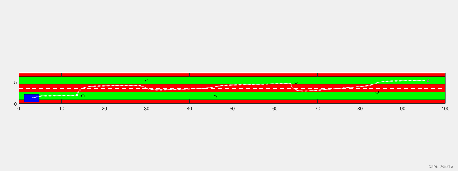
4、来自 jubobolv369 的MATLAB版本程序
(1)程序来源:人工势场法–路径规划–原理–matlab代码【点击可跳转】
(2)程序如下所示:
clc;
clear;
close all;
%% 基本信息、常数等设置
eta_ob=25;          %计算障碍物斥力的权益系数
eta_goal=10;        %计算障目标引力的权益系数
eta_border=25;      %车道边界斥力权益系数
n=1;                 %计算障碍物斥力的常数
border0=20;          %斥力作用边界
max_iter=1000;        %最大迭代次数
step=0.3;            %步长

car_width=1.8;         %车宽
car_length=3.5;      %车长
road_width=3.6;      %道路宽
road_length=100;      %道路长

%% 起点、障碍物、目标点的坐标、速度信息

P0=[3 1.3 1 1];               %横坐标 纵坐标 x方向分速度 y方向分速度
Pg=[road_length-4 5.4 0 0];
Pob=[15 1.8;
     30 5.4;
     46 1.6;
     65 5.0;
     84 2.7;]

 %% 未达目标附近前不断循环
 Pi=P0;
 i=1;
 while sqrt((Pi(1)-Pg(1))^2+(Pi(2)-Pg(2))^2)>1
     if i>max_iter
         break;
     end
     %计算每个障碍物与当前车辆位置的向量(斥力)、距离、单位向量
     for j=1:size(Pob,1)
         vector(j,:)=Pi(1,1:2)-Pob(j,1:2);
         dist(j,:)=norm(vector(j,:));
         unit_vector(j,:)=[vector(j,1)/dist(j,:) vector(j,2)/dist(j,:)];
     end

     %计算目标与当前车辆位置的向量(引力)、距离、单位向量
     max=j+1;
     vector(max,:)=Pg(1,1:2)-Pi(1,1:2);
     dist(max,:)=norm(vector(max,:));
     unit_vector(max,:)=[vector(max,1)/dist(max,:) vector(max,2)/dist(max,:)];

     %计算每个障碍物的斥力
     for j=1:size(Pob,1)
        if dist(j,:)>=border0
            Fre(j,:)=[0,0];
        else
            %障碍物斥力指向物体
            Fre_abs_ob=eta_ob*(1/dist(j,:)-1/border0)*(dist(max)^n/dist(j,:)^2);
            Fre_ob=[Fre_abs_ob*unit_vector(j,1) Fre_abs_ob*unit_vector(j,2)];
            %障碍物斥力 指向目标
            Fre_abs_g=n/2*eta_ob*(1/dist(j,:)-1/border0)^2*dist(max)^(n-1);
            Fre_g=[Fre_abs_g*unit_vector(max,1) Fre_abs_g*unit_vector(max,2)];
            Fre(j,:)=Fre_ob+Fre_g;
        end
     end

     if Pi(2)>=(road_width-car_width)/2 && Pi(2)< road_width/2   %下绿色下区域
         Fre_edge=[0,eta_border*norm(Pi(1,3:4))*(exp(road_width/2)-Pi(2))];
     elseif Pi(2)>= road_width/2 &&  Pi(2)<= (road_width+car_width)/2   %下绿色上区域
         Fre_edge=[0,-1/3*eta_border*Pi(2)^2];
     elseif Pi(2)>=(3*road_width-car_width)/2 && Pi(2)<= 3*road_width/2   %上绿色下区域
         Fre_edge=[0,1/3*eta_border*(3*road_width/2-Pi(2))^2];
     elseif Pi(2)>=3*road_width/2 && Pi(2)<= (3*road_width+car_width)/2    %上绿色上区域
         Fre_edge=[0,eta_border*norm(Pi(1,3:4))*(exp(Pi(2)-3*road_width/2))];
     else
         Fre_edge=[0 0];
     end

     Fre=[sum(Fre(:,1))+Fre_edge(1) sum(Fre(:,2))+Fre_edge(2)];
     %计算引力
     Fat=[eta_goal*dist(max,1)*unit_vector(max,1) eta_goal*dist(max,1)*unit_vector(max,2)];

     F_sum=[Fre(1)+Fat(1),Fre(2)+Fat(2)];
     unit_vector_sum(i,:)=F_sum/norm(F_sum);

     Pi(1,1:2)= Pi(1,1:2)+step*unit_vector_sum(i,:);

     path(i,:)= Pi(1,1:2);
     i=i+1;
 end
 %% 画图
figure(1)
%下车道下红色区域
fill([0,road_length,road_length,0],[0,0,(road_width-car_width)/2,(road_width-car_width)/2],[1,0,0]);
hold on
%下车道上红色区域,上车道下红色区域
fill([0,road_length,road_length,0],[(road_width+car_width)/2,(road_width+car_width)/2,...
     (3*road_width-car_width)/2,(3*road_width-car_width)/2],[1,0,0]);
%下车道绿色区域
fill([0,road_length,road_length,0],[(road_width-car_width)/2,(road_width-car_width)/2,...
     (road_width+car_width)/2,(road_width+car_width)/2],[0,1,0]);

%上车道绿色区域
fill([0,road_length,road_length,0],[(3*road_width-car_width)/2,(3*road_width-car_width)/2,...
     (3*road_width+car_width)/2,(3*road_width+car_width)/2],[0,1,0]);
%上车道上红色区域
fill([0,road_length,road_length,0],[ (3*road_width+car_width)/2,(3*road_width+car_width)/2,2*road_width,2*road_width],[1,0,0]);
%路面中心线、边界线
plot([0,road_length],[road_width,road_width],'w--','linewidth',2);
plot([0,road_length],[2*road_width,2*road_width],'w','linewidth',2);
plot([0,road_length],[0,0],'w','linewidth',2);

%障碍物、目标
plot(Pob(:,1),Pob(:,2),'ko');
plot(Pg(1),Pg(2),'mp');
%车
fill([P0(1)-car_length/2,P0(1)+car_length/2,P0(1)+car_length/2,P0(1)-car_length/2],...
     [P0(2)-car_width/2,P0(2)-car_width/2,P0(2)+car_width/2,P0(2)+car_width/2],[0,0,1]);

 plot(path(:,1),path(:,2),'w.');

axis equal
set(gca,'XLim',[0 road_length])
set(gca,'YLim',[0 2*road_width])
(3)上述程序运行结果示例:
文章出处登录后可见!