基于Lasso回归的实证分析
一、背景
随着信息化时代的到来,对如证券市场交易数据、多媒体图形图像视频数据、航天航空采集数据、生物特征数据等数据维度远大于样本量个数的高维数据分析逐渐占据重要地位。而在分析高维数据过程中碰到最大的问题就是维数膨胀,也就是通常所说的“维数灾难”问题。研究表明,随着维数的增长,分析所需的空间样本数会呈指数增长。并且在高维数据空间中预测将变得不再容易,同时还容易导致模型的过拟合。因此为了应对高维数据中的维数灾难所带来的过拟合问题,其中一条解决思路是进行数据降维。在数据降维的方法中,Lasso方法是一种既适用于线性情况也适用于非线性情况的数据降维方法。
二、理论基础
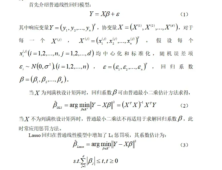
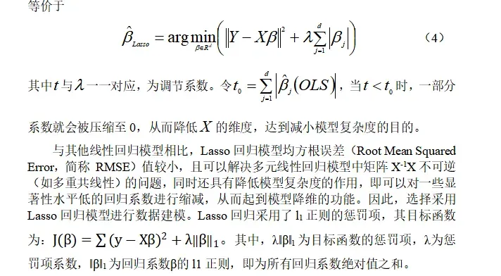
Lasso方法是基于惩罚方法对样本数据进行变量选择,通过对原本普通线性回归模型的系数进行压缩,将原本很小的系数直接压缩至0,从而将这部分系数所对应的变量视为非显著性变量,将不显著的变量直接舍弃,达到简化模型的目的。
三、数据来源
《统计学习导论-基于R应用》的信用卡违约数据
四、变量选择
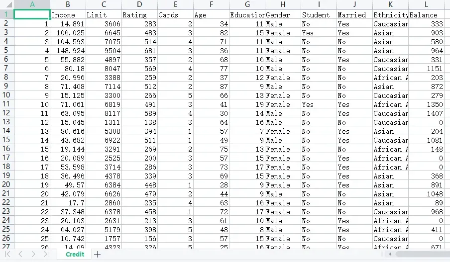
1.被解释变量:Balance信用卡账户余额,记为Y。
2.解释变量:
(1)Income:收入情况。
(2)Limit:信用额度。
(3)Rating:信用等级。
(4)Cards:信用卡数量。
(5)Age:年龄。
(6)Education:判断受教育程度。
(7)Gender:判断性别。
(8)Student:判断是否为学生。
(9)Married:判断婚姻状况。
(10)Ethnicity:划分种族。
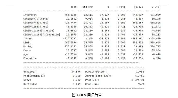
五、建模步骤
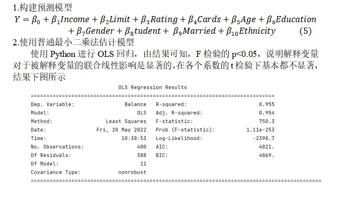
3.使用Lasso回归进行变量选择
利用Lasso回归模型的交叉验证确定最佳的惩罚项系数λ,基于最佳的λ值重新构建Lasso回归模型来确定解释变量的系数。
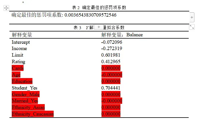
使用交叉验证来选择最佳的调整参数,使用均方误差进行评估,故模型预测准确率较高,均方误差较小(MSE: 0.0012621555901723037)。
绘制正则化路径,可知变量进入模型的先后顺序Rating、Limit、Income、Student_Yes,说明这四个变量对信用卡账户余额的影响效果显著
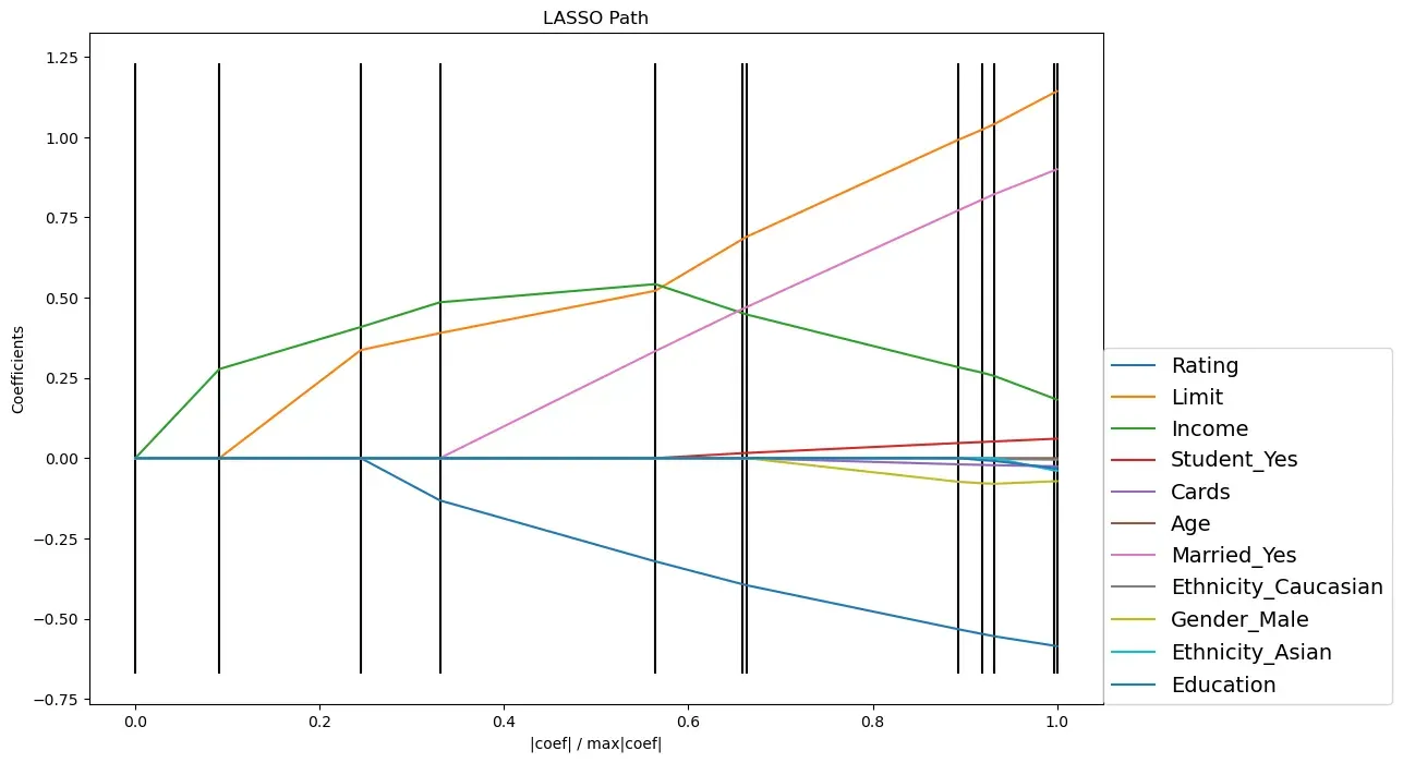
前四个进入模型的自变量: [‘Rating’ ‘Limit’ ‘Income’ ‘Student_Yes’]
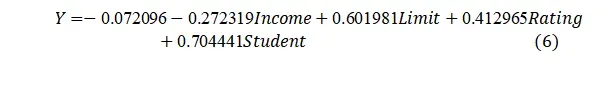
从拟合结果可知,信用卡账户余额(Balance)Y预测模型中系数系数有7个为0,分别为Cards、Age、Education、Gender_Male、Married_Yes、Ethnicity_Asian、Ethnicity_Caucasian,说明信用卡数量、年龄、受教育程度、性别、婚姻状况、种这五个变量对信用卡账户余额没有显著意义,故Y的回归模型可表达为:
六、Python实现代码
# -*- coding: utf-8 -*-
"""
Created on Thu May 19 19:30:29 2022
@author: DELL
"""
'''
Lasso变量选择,某些自变量系数估计值压缩为零。
首先构建包含所有自变量的的模型,注意要对属性类型进行因子化,即转换成哑变量。
'''
from sklearn.preprocessing import StandardScaler
import statsmodels.formula.api as smf
import statsmodels.api as sm
import seaborn as sns
import numpy as np
import pandas as pd
import matplotlib.pyplot as plt
import patsy
pd.set_option("display.max_rows",None)
pd.set_option("display.max_columns",None)
pd.set_option("display.expand_frame_repr",False)
data = pd.read_csv(r'E:\研究生\关于课程\研一下\高维函数型数据分析\作业\第二次作业\datashine-master\data\credit.csv',index_col=0)
print('数据形状:',data.shape)
print('\n数据示例:')
data.head(10)
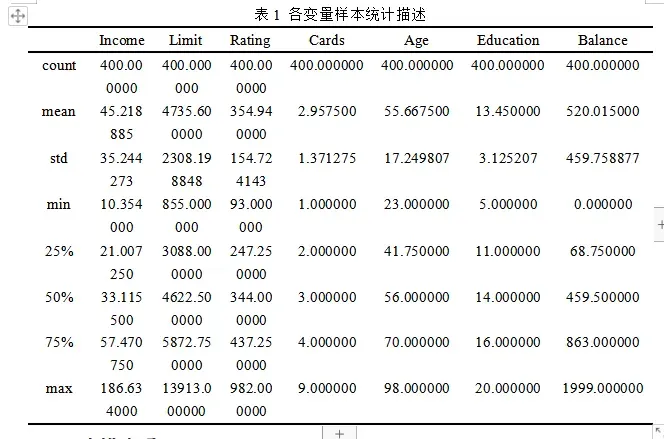
print("各样本统计量描述")
print(data.describe())
X = data.copy()
scaler = StandardScaler()
#数值型数据进行标准化
X[['Income','Limit','Rating','Cards','Age','Education']]=scaler.fit_transform(
X[['Income','Limit','Rating','Cards','Age','Education']])
X['Balance']=data['Balance']
###模型包含了所有自变量,对于因子变量通过patsy的C函数转换成category类别变量
#C为设计矩阵
formula = 'Balance~Income+Limit+Rating+Cards+Age+Education+C(Gender)\
+C(Student)+C(Married)+C(Ethnicity)'
#构建简单的线性回归模型
#普通最小二乘法,用标准化后的数据进行拟合
model=smf.ols(formula,data=X)
print(model)
result_ols=model.fit()
#拟合后的统计描述
print(result_ols.summary())
#lasso回归
#最优 λ参数选择
#选择fit_regularized函数参数 α 的最优值
X1=data.copy()
dummies1 = pd.get_dummies(X1.Student, prefix='Student')
dummies2 = pd.get_dummies(X1.Gender, prefix='Gender')
dummies3 = pd.get_dummies(X1.Married, prefix='Married')
dummies4 = pd.get_dummies(X1.Ethnicity, prefix='Ethnicity')
X1=X1.drop('Student',axis=1).join(dummies1)
X1=X1.drop('Gender',axis=1).join(dummies2)
X1=X1.drop('Married',axis=1).join(dummies3)
X1=X1.drop('Ethnicity',axis=1).join(dummies4)
X1=X1.drop('Student_No',axis=1)
X1=X1.drop('Gender_Female',axis=1)
X1=X1.drop('Married_No',axis=1)
X1=X1.drop('Ethnicity_African American',axis=1)
scaler = StandardScaler()
X1[['Income','Limit','Rating','Cards','Age','Education','Balance']]=scaler.fit_transform( \
X1[['Income','Limit','Rating','Cards','Age','Education','Balance']])
#X1['Balance']=data['Balance']
dummies1,X1.head()
'''
Lasso的Lambda最优值选择。
使用sklearn机器学习库相关函数,比如LassoCV等。sklearn中对应的模型为LASSO以及带自动筛选alpha值得LASSOCV模型
'''
import pandas as pd
import numpy as np
from sklearn import model_selection
from sklearn.linear_model import Lasso, LassoCV, LassoLarsIC
from sklearn.metrics import mean_squared_error
predictors=['Income','Limit','Rating','Cards','Age','Education',
'Student_Yes','Gender_Male','Married_Yes',
'Ethnicity_Asian','Ethnicity_Caucasian']
x_train,x_test,y_train,y_test=model_selection.train_test_split(X1[predictors],
X1.Balance,test_size=0.2,
random_state=1234)
#构造不同的lambda值
#等比数列
Lambdas=np.logspace(-5,10,200)
#设置交叉验证的参数,使用均方误差评估
lasso_cv=LassoCV(alphas=Lambdas,normalize=False,cv=10,max_iter=10000)
lasso_cv.fit(x_train,y_train)
print("确定最佳的惩罚项系数:",lasso_cv.alpha_)
#基于最佳lambda值建模
lasso=Lasso(alpha=lasso_cv.alpha_,normalize=True,max_iter=10000)
lasso.fit(x_train,y_train)
#打印回归系数
print('系数列表:',pd.DataFrame(index=['Intercept']+x_train.columns.tolist(),columns=[''],
data=[lasso.intercept_]+lasso.coef_.tolist()))
#模型评估
lasso_pred=lasso.predict(x_test)
#均方误差
# Balance_80=y_test
# print(Balance_80)
# Balance_predict_80=pd.Series(lasso_pred)
# print(Balance_predict_80)
MSE=mean_squared_error(y_test,lasso_pred)/80
print('\nMSE:',MSE,'\n\n最优lambda:',lasso_cv.alpha_)
import matplotlib.pyplot as plt
from sklearn import linear_model
X2=x_train
Y2=y_train
X3=np.array(X2)
Y3=np.array(Y2)
#使用LARS的Lasso路径LARS算法几乎完全提供了沿着正则化参数的系数的完整路径,
# 因此常见的操作是使用包括所有检索的路径的 lars_path函数。
#是Lasso模型在引入了LARS算法后的一种新的实现。
#这不同于基于坐标下降的实现,它会产生一个精确的解,作为其系数的范数的分段线性函数。
_, n3, coefs = linear_model.lars_path(X3, Y3, method='lasso',verbose=True)
print("进入模型的自变量对应的索引值:",n3)
xx = np.sum(np.abs(coefs.T), axis=1)
xx /= xx[-1]
plt.figure(figsize=[12,8])
plt.plot(xx, coefs.T)
ymin, ymax = plt.ylim()
plt.vlines(xx, ymin, ymax, linestyle='dashed')
plt.xlabel('|coef| / max|coef|')
plt.ylabel('Coefficients')
plt.title('LASSO Path')
plt.axis('tight')
plt.legend(np.array(predictors)[n3],fontsize=14,bbox_to_anchor=(1, 0), loc=3, borderaxespad=0)
print('前四个进入模型的自变量:',np.array(predictors)[n3[0:4]])
plt.savefig('正则化路径图.png',bbox_inches='tight')
plt.show()
文章出处登录后可见!