一:boston数据集
Boston数据集各个特征的含义如下:
| 特征值 | 特征值含义 |
| CRIM | 城镇人均犯罪率 |
| ZN | 住宅用地所占比例 |
| INDUS | 城镇中非住宅用地所占比例 |
| CHAS | 虚拟变量,用于回归分析 |
| NOX | 环保指数 |
| RM | 每栋住宅的房间数 |
| AGE | 1940 年以前建成的自住单位的比例 |
| DIS | 距离 5 个波士顿的就业中心的加权距离 |
| RAD | 距离高速公路的便利指数 |
| TAX | 每一万美元的不动产税率 |
| PTRATIO | 城镇中的教师学生比例 |
| B | 城镇中的黑人比例 |
| LSTAT | 地区中有多少房东属于低收入人群 |
| MEDV | 自住房屋房价中位数(也就是均价) |
波士顿房价数据集包括506个样本,每个样本包括12个特征变量和该地区的平均房价,房价显然和多个特征变量相关,先选择亿元线性回归与多个特征建立线性方程,观察模型预测的好坏,再选择多元线性回归进行房价预测。
建立线性模型

二:boston数据处理及模型建立
2.1加载boston数据集
import pandas as pd
import numpy as np
import matplotlib
matplotlib.rcParams[‘font.sans-serif’] = [‘SimHei’]
matplotlib.rcParams[‘font.family’] = ‘sans-serif’
matplotlib.rcParams[‘axes.unicode_minus’] = False
import matplotlib.pyplot as plt
from sklearn import datasets
# 获取数据
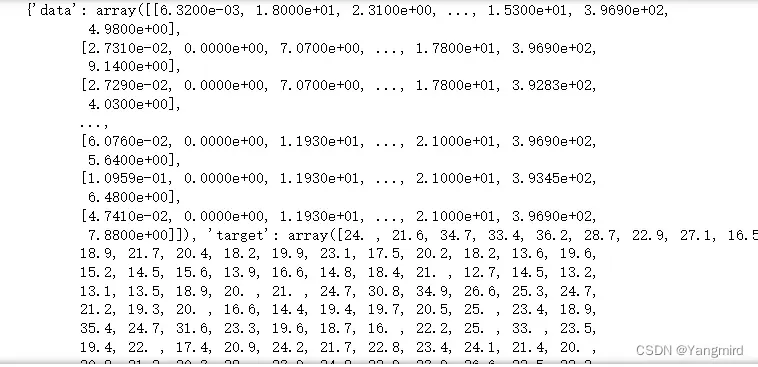
boston = datasets.load_boston()
print(boston)
boston_df = pd.DataFrame(boston.data, columns=boston.feature_names)
boston_df[‘MEDV’] = boston.target # 房价—–y
查看数据:
# 查看数据是否存在空值,从结果来看数据不存在空值。
boston_df.isnull().sum()
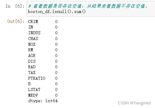
可以看出,boston数据集中有14个特征,并且没有缺失值,所以不用做缺失值处理,其中’MEDV’作为目标值。
# 查看数据大小
boston_df.shape
![]()
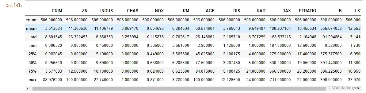
# 查看数据的描述信息,在描述信息里可以看到每个特征的均值,最大值,最小值等信息。
boston_df.describe()
# 看看各个特征中是否有相关性,判断一下用哪种模型比较合适
import seaborn as sns
plt.figure(figsize=(12,8))
sns.heatmap(boston_df.corr(), annot=True, fmt=’.2f’,cmap=’PuBu’)
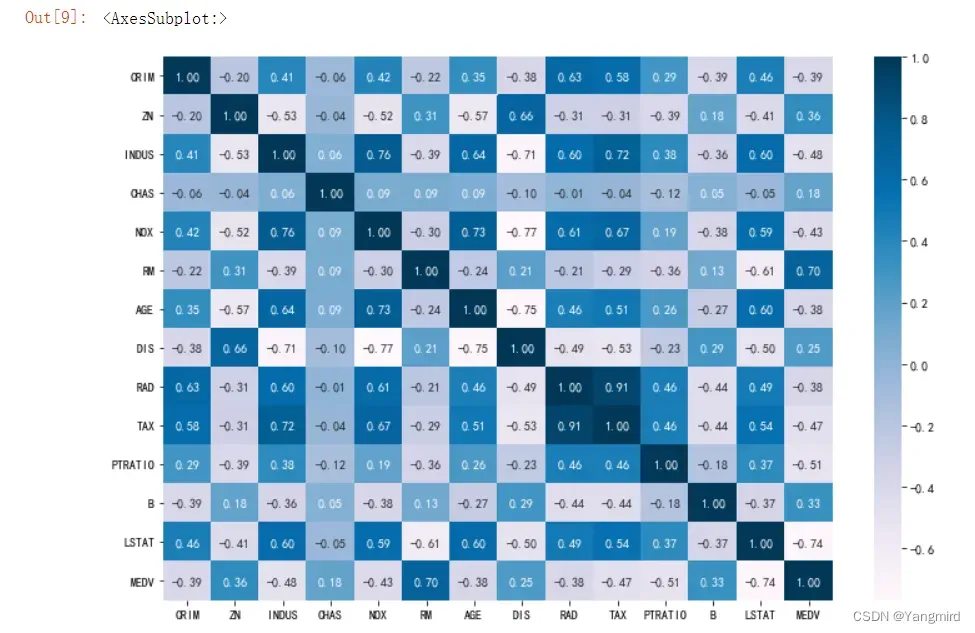
从上图可以看出数据不存在相关性较小的属性,也不用担心共线性,所以可以用线性回归模型去预测。
2.2 画出各个特征与MEDV房价的散点图
# 各个特征和MEDV房价的散点图
boston_df_xTitle=[‘CRIM’,’ZN’,’INDUS’,’CHAS’,’NOX’,’RM’,’AGE’,’DIS’,’RAD’,’TAX’,’PTRATIO’,’B’,’LSTAT’]
for i in range(0,len(boston_df_xTitle)):
plt.figure(facecolor=’white’)
plt.scatter(boston_df[str(boston_df_xTitle[i])], boston_df[‘MEDV’], s=30, edgecolor=’white’)
plt.title(str(boston_df_xTitle[i])+’——–MEDV’)
plt.xlabel(str(boston_df_xTitle[i]))
plt.ylabel(‘MEDV房价’)
plt.show()
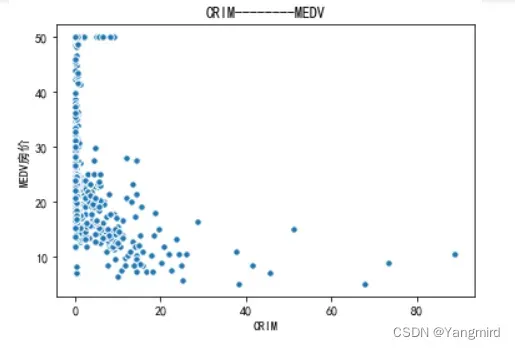
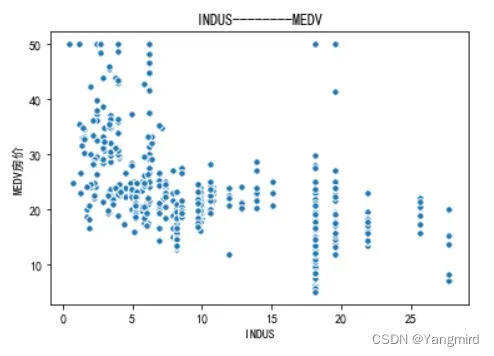
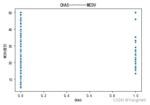
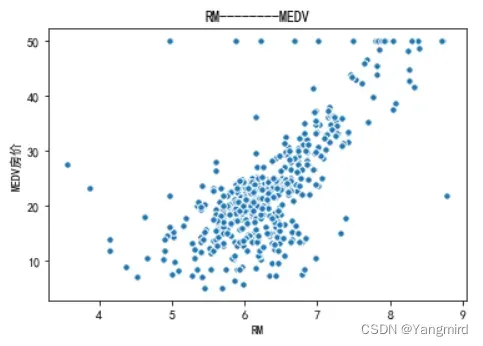
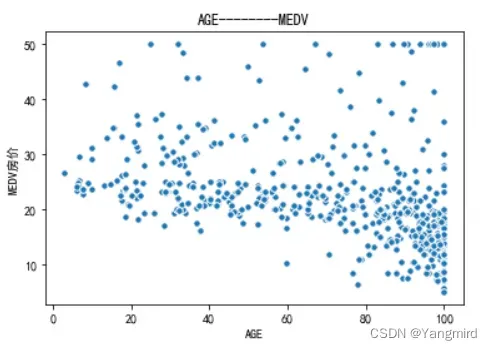
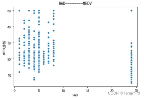
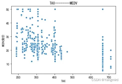
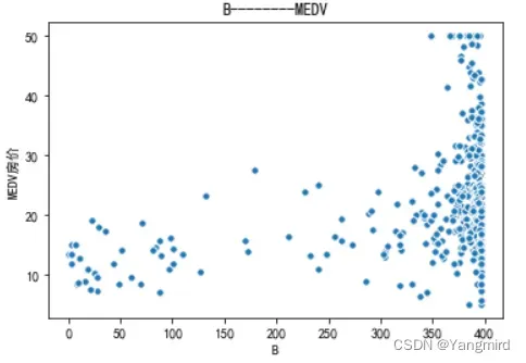
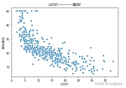
从上图可以看出’RM’,’LSTAT’,’CRIM’这三个特征值与房价存在一定的相关性,所以选择该三个特征作为特征值,移除其余不相关的特征值。
# 定义目标值和特征值
# 分析房屋的’RM’, ‘LSTAT’,’CRIM’ 特征与MEDV的相关性性,所以,将其余不相关特征移除
new_boston_df = boston_df[[‘LSTAT’, ‘CRIM’, ‘RM’, ‘MEDV’]]
# print(‘describe: ‘)
# new_boston_df.describe()
# 目标值
y = np.array(new_boston_df[‘MEDV’])
# drop函数默认删除行,列需要加axis=1
new_boston_df = new_boston_df.drop([‘MEDV’], axis=1)
# 特征值
X = np.array(new_boston_df)
2.3划分训练集和测试集
由于数据没有null值,并且,都是连续型数据,所以暂时不用对数据进行过多的处理,不够既然要建立模型,首先就要进行对boston数据集分为训练集和测试集,取出了大概百分之30的数据作为测试集,剩下的百分之70为训练集
# 划分训练集和测试集
from sklearn.model_selection import train_test_split
# 70%用于训练,30%用于测试
X_train, X_test, y_train, y_test = train_test_split(X, y, test_size=0.2, random_state=10)
print(X_train.shape, X_test.shape, y_train.shape, y_test.shape)
![]()
2.4建立线性回归模型
# 线性回归————————————————-
from sklearn.linear_model import LinearRegression
from sklearn.preprocessing import StandardScaler
lr = LinearRegression()
# ss=StandardScaler()
# 使用训练数据进行参数估计
lr.fit(X_train, y_train)
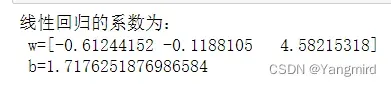
# 输出线性回归的系数
print(‘线性回归的系数为:\n w=%s\n b=%s ‘ % (lr.coef_, lr.intercept_))
lr_reg_pre=lr.predict(X_test)
# ———————————————————–
2.5计算MAE和MSE
# 进行预测
# 使用测试数据进行回归预测
y_test_pred = lr.predict(X_test)
print(‘y_test_pred:\n’, y_test_pred)
# 训练数据的预测值
y_train_pred = lr.predict(X_train)
print(‘y_train_pred : \n ‘, y_train_pred)
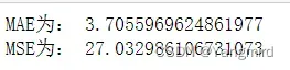
# 计算平均绝对误差MAE
train_MAE=mean_absolute_error(y_train,y_train_pred)
print(‘MAE为:’,train_MAE)
# 计算均方误差MSE
train_MSE=mean_squared_error(y_train,y_train_pred) # 训练值与训练预测值之间的对比
print(‘MSE为:’,train_MSE)
# 绘制MAE和MSE图
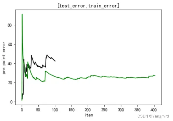
2.6画出学习曲线
from sklearn.model_selection import learning_curve,ShuffleSplit
def plot_learning_curve(plt,estimator,title,X,y,
ylim=None,cv=None,n_jobs=1,train_sizes=np.linspace(.1,1.0,5)):
plt.title(title)
if ylim is not None:
plt.ylim(ylim)
plt.xlabel(“Training examples”)
plt.ylabel(“Score”)
train_sizes,train_scores,test_scores=learning_curve(estimator,X,y,cv=cv,n_jobs=n_jobs,train_sizes=train_sizes)
train_scores_mean=np.mean(train_scores,axis=1)
train_scores_std=np.std(train_scores,axis=1)
test_scores_mean=np.mean(test_scores,axis=1)
test_scores_std=np.std(test_scores,axis=1)
plt.grid()
plt.fill_between(train_sizes,train_scores_mean-train_scores_std,train_scores_mean+train_scores_std,alpha=0.1,color=”r”)
plt.fill_between(train_sizes,test_scores_mean-test_scores_std,test_scores_mean+test_scores_std,alpha=0.1,color=”g”)
plt.plot(train_sizes,train_scores_mean,’o–‘,color=”r”,label=”Training scores”)
plt.plot(train_sizes,test_scores_mean,’o-‘,color=”g”,label=”Cross-validation score”)
plt.legend(loc=”best”)
return plt
cv=ShuffleSplit(n_splits=10,test_size=0.2,random_state=0)
plt.figure(figsize=(10,6))
plot_learning_curve(plt,lr,”Learn Curve for LinearRegression”,new_boston_df,y,ylim=None,cv=cv)
plt.show()
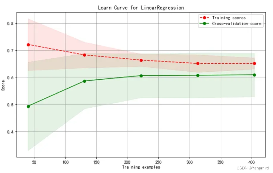
可以看出,模型有些欠拟合,需要优化,考虑使用二项式、三项式进行优化。
三:模型优化及结果分析
3.1模型优化
# 定义划分数据集函数
def split_data():
X=boston.data
y=boston.target
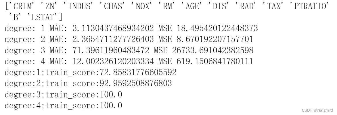
print(boston.feature_names)
X_train, X_test, y_train, y_test = train_test_split(X, y, test_size=0.2, random_state=2)
return (X, y, X_train, X_test, y_train, y_test)
# 定义MAE函数
def mae_value(y_train,y_train_pred):
n=len(y_train)
mae=mean_absolute_error(y_train,y_train_pred)
return mae
# 定义MSE函数
def mse_value(y_train,y_train_pred):
n=len(y_train)
mse=mean_squared_error(y_train,y_train_pred)
return mse
# 定义多项式模型函数
from sklearn.preprocessing import PolynomialFeatures
from sklearn.pipeline import Pipeline
def polynomial_regression(degree=1):
polynomial_features=PolynomialFeatures(degree=degree,include_bias=False)
# 模型开启数据归一化
linear_regression_model=LinearRegression(normalize=True)
model=Pipeline([(“polynomial_features”, polynomial_features),
(“linear_regression”, linear_regression_model)])
return model
# 训练模型
def train_model(X_train, X_test, y_train, y_test,degrees):
res=[]
for degree in degrees:
model=polynomial_regression(degree)
model.fit(X_train,y_train)
train_score=model.score(X_train,y_train)*100
test_score = model.score(X_test, y_test)*100
res.append({‘model’:model,’degree’:degree,’train_score’:train_score,’test_score’:test_score})
y_test_predict=model.predict(X_test)
mae=mae_value(y_test,y_test_predict)
mse=mse_value(y_test,y_test_predict)
print(“degree:”,degree, “MAE:”,mae,”MSE”,mse)
for r in res:
print(“degree:{};train_score:{}”.format(r[“degree”],r[“train_score”],r[“test_score”]))
return res
# 定义画出学习曲线的函数
from sklearn.model_selection import learning_curve
def plot_learning_curve(plt,estimator,title,X,y,ylim=None,cv=None,n_jobs=1,train_sizes=np.linspace(.1,1.0,5)):
plt.title(title)
if ylim is not None:
plt.ylim(ylim)
plt.xlabel(“Training examples”)
plt.ylabel(“Score”)
train_sizes,train_scores,test_scores=learning_curve(estimator,X,y,cv=cv,n_jobs=n_jobs,train_sizes=train_sizes)
train_scores_mean=np.mean(train_scores,axis=1)
train_scores_std=np.std(train_scores,axis=1)
test_scores_mean=np.mean(test_scores,axis=1)
test_scores_std=np.std(test_scores,axis=1)
plt.grid()
plt.fill_between(train_sizes,train_scores_mean-train_scores_std,train_scores_mean+train_scores_std,alpha=0.1,color=”r”)
plt.fill_between(train_sizes,test_scores_mean-test_scores_std,test_scores_mean+test_scores_std,alpha=0.1,color=”g”)
plt.plot(train_sizes,train_scores_mean,’o–‘,color=”r”,label=”Training scores”)
plt.plot(train_sizes,test_scores_mean,’o-‘,color=”g”,label=”Cross-validation score”)
plt.legend(loc=”best”)
return plt
# 定义1、2、3次多项式
degrees=[1,2,3,4]
# 划分数据集
X, y, X_train, X_test, y_train, y_test = split_data()
#训练模型,并打印train score
res = train_model(X_train, X_test, y_train, y_test, degrees)
# 画出学习曲线
from sklearn.model_selection import ShuffleSplit
cv=ShuffleSplit(n_splits=10, test_size=0.2, random_state=0)
plt.figure(figsize=(10,6))
for index,data in enumerate(res):
plot_learning_curve(plt,data[“model”],”degree%d”%data[“degree”],X,y,cv=cv)
plt.show()
3.2结果分析
模型优化结果如下:
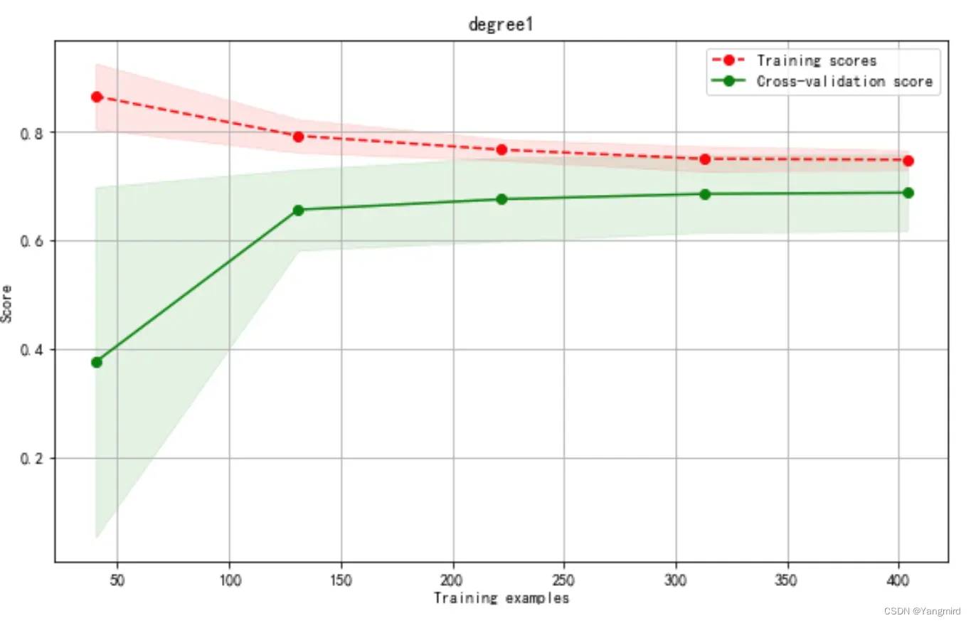
Degree=1时学习曲线如下:
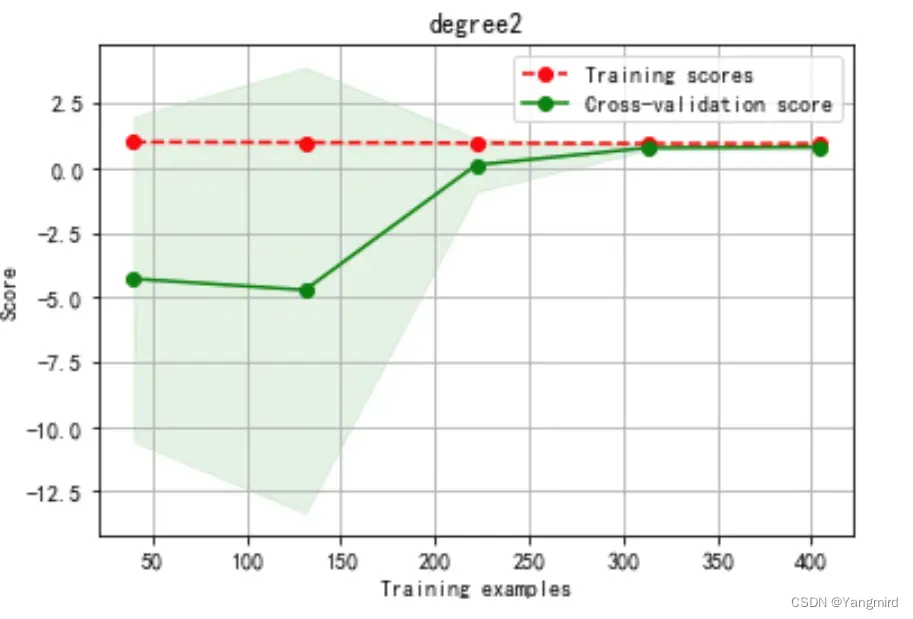
Degree=2时学习曲线如下:
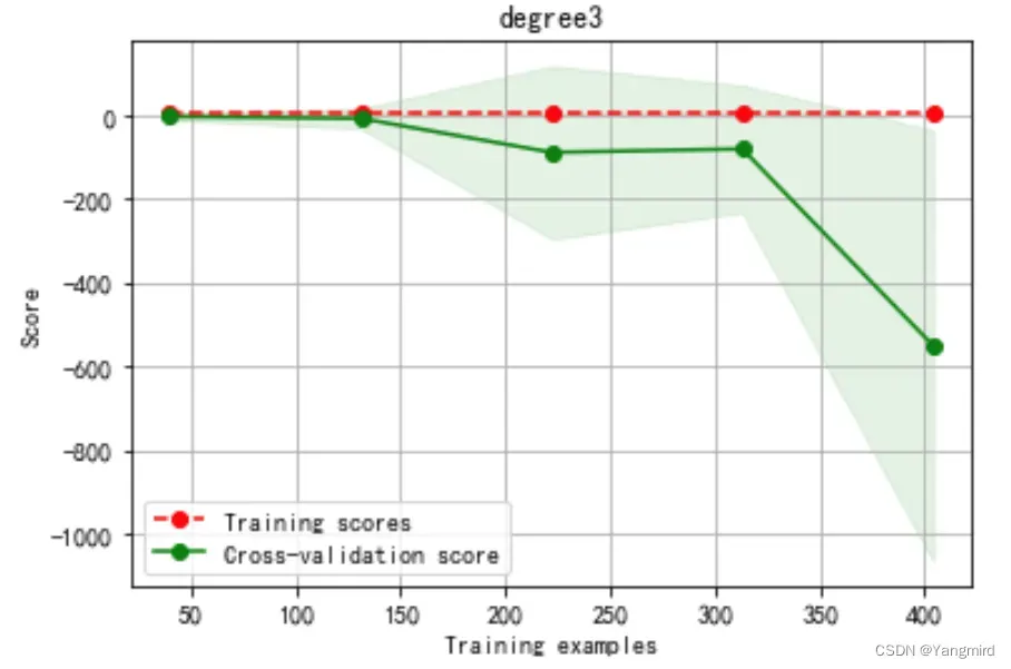
Degree=3时学习曲线如下:
Degree=4时学习曲线如下:
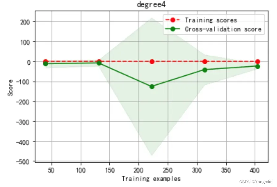
根据上述模型优化结果分析可知,二次多项式效果较好,训练准确度达到了92.9%,MAE=2.36,MSE=8.67,比一次多项式的训练准确度72.8%要更准确。
文章出处登录后可见!