文章目录
- 一,旅行商问题QUBO的两种实现
- 二,方式一:取余操作
- 三、方式二:独立矩阵
- 总结
一,旅行商问题QUBO的两种实现
提示:上篇已经讲过了旅行商问题的QUBO建模,这里直接讲两种编程实现:
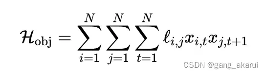
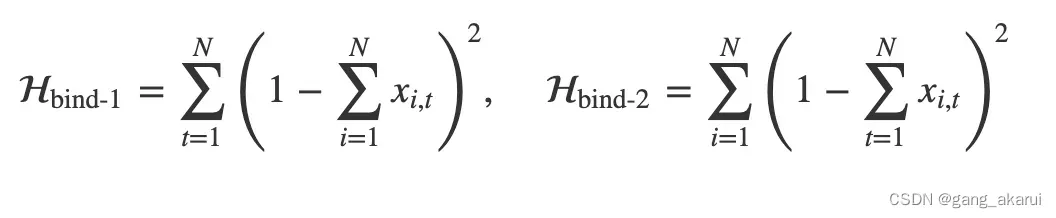
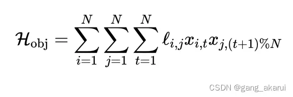
看过上篇的读者应该已经注意到,因为旅行商问题需要最终返回到初始点的。所以,下面👇的目标函数里,循环进行到时,最后一个
应该确定回到初始点的。
-
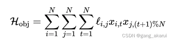
方式一:使用取余操作符%,在
时,这样的话
=1,也就相当于最后一个时间步回到了初始点。
-
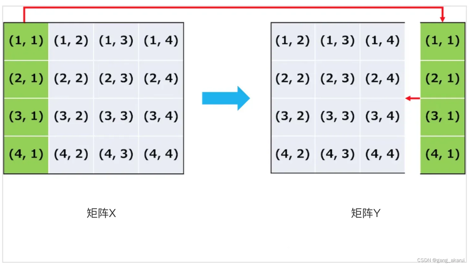
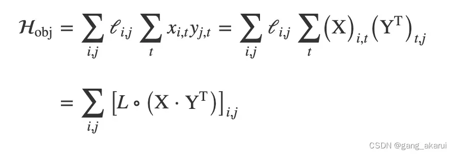
方式二:把
和
对应的数值矩阵,分为独立的两个矩阵。具体来说,
,从式子上看,有点难以理解,大家可以看下面的图示。其实就是把矩阵X的第一列,转移到最后一列。
提示:下面分别献上python实现:
二,方式一:取余操作
这里代码复制于下面的链接,这里只讲解QUBO部分的代码:
https://github.com/recruit-communications/pyqubo/blob/master/notebooks/TSP.ipynb
旅行问题的QUBO的定义:
%matplotlib inline
from pyqubo import Array, Placeholder, Constraint
import matplotlib.pyplot as plt
import networkx as nx
import numpy as np
import neal

# 地点名和坐标 list[("name", (x, y))]
cities = [
    ("a", (0, 0)),
    ("b", (1, 3)),
    ("c", (3, 2)),
    ("d", (2, 1)),
    ("e", (0, 1))
]

n_city = len(cities)
下面实现约束部分:
# ‘BINARY’代表目标变量时0或1
x = Array.create('c', (n_city, n_city), 'BINARY')

# 约束① : 每个时间步只能访问1个地点
time_const = 0.0
for i in range(n_city):
    # Constraint(...)函数用来定义约束项
    time_const += Constraint((sum(x[i, j] for j in range(n_city)) - 1)**2, label="time{}".format(i))

# 约束② : 每个地点只能经过1次
city_const = 0.0
for j in range(n_city):
    city_const += Constraint((sum(x[i, j] for i in range(n_city)) - 1)**2, label="city{}".format(j))
接下来是目标函数:
# 目标函数的定义

distance = 0.0
for i in range(n_city):
    for j in range(n_city):
        for k in range(n_city):
            d_ij = dist(i, j, cities)
            distance += d_ij * x[k, i] * x[(k+1)%n_city, j]
最后就是整体的Hamiltonian量定义和输出采样结果。
# 总体的Hamiltonian,这里的A代表约束项的惩罚系数,数值自由指定
A = Placeholder("A")
H = distance + A * (time_const + city_const)

# 求BQM
model = H.compile()
feed_dict = {'A': 4.0}
bqm = model.to_bqm(feed_dict=feed_dict)


sa = neal.SimulatedAnnealingSampler()
# 这里要注意,退火算法是要采样足够的次数,从中取占比最高的结果作为最优解
sampleset = sa.sample(bqm, num_reads=100, num_sweeps=100)

# Decode solution
decoded_samples = model.decode_sampleset(sampleset, feed_dict=feed_dict)
best_sample = min(decoded_samples, key=lambda x: x.energy)


# 如果指定参数only_broken=True,则只会返回损坏的约束。
# 如果best_sample长度为0,就代表没有损坏的约束项,也就满足最优解了。
num_broken = len(best_sample.constraints(only_broken=True))
if num_broken == 0:
	print(best_sample.sample)
三、方式二:独立矩阵
这里的实现复制于以下文章:
https://qiita.com/yufuji25/items/0425567b800443a679f7
import neal
import numpy as np
import networkx as nx
import matplotlib.pyplot as plt
from pyqubo import Array, Placeholder
from scipy.spatial.distance import cdist


def construct_graph(n_pos:int):
    """ construct complete graph """
    pos = nx.spring_layout(nx.complete_graph(n_pos))
    coordinates = np.array(list(pos.values()))
    G = nx.Graph(cdist(coordinates, coordinates))
    nx.set_node_attributes(G, pos, "pos")
    return G
整体Hamiltonian量: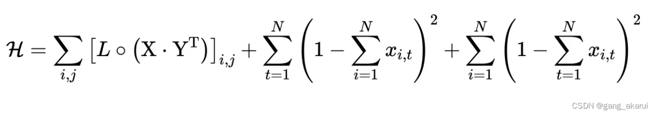
def create_hamiltonian(G:nx.Graph):
    """ create QUBO model from graph structure """

    # generate QUBO variable
    n_pos = G.number_of_nodes()
    X = np.array(Array.create("X", shape = (n_pos, n_pos), vartype = "BINARY"))

    # construct `Y` matrix
    Xtmp = np.concatenate([X, X[:, 0].reshape(-1, 1)], axis = 1)
    Y = np.delete(Xtmp, 0, 1)

    # Distance matrix
    L = np.array(nx.adjacency_matrix(G).todense())

    # return hamiltonian
    Hbind1 = np.sum((1 - X.sum(axis = 0)) ** 2)
    Hbind2 = np.sum((1 - X.sum(axis = 1)) ** 2)
    Hobj = np.sum(X.dot(Y.T) * L)
    H = Hobj + Placeholder("a1") * Hbind1 + Placeholder("a2") * Hbind2

    return H.compile()
求解并输出结果:
def decode(response, Gorigin:nx.Graph):
    """ return output graph generated from response """

    # derive circuit
    solution = min(response.record, key = lambda x: x[1])[0]
    X = solution.reshape((num_pos, num_pos))
    circuit = np.argmax(X, axis = 0).tolist()
    circuit.append(circuit[0])

    # generate output graph structure
    Gout = nx.Graph()
    Gout.add_edges_from(list(zip(circuit, circuit[1:])))
    positions = nx.get_node_attributes(Gorigin, "pos")
    nx.set_node_attributes(Gout, positions, "pos")

    return Gout


def draw_graph(G:nx.Graph, **config):
    """ drawing graph """
    plt.figure(figsize = (5, 4.5))
    nx.draw(G, nx.get_node_attributes(G, "pos"), **config)
    plt.show()


# configuration for drawing graph
config = {"with_labels":True, "node_size":500, "edge_color":"r", "width":1.5,
          "node_color":"k", "font_color":"w", "font_weight":"bold"}

# construct complete graph
num_pos = 8
G = construct_graph(num_pos)
draw_graph(G, **config)

# sampling
model = create_hamiltonian(G)
qubo, offset = model.to_qubo(feed_dict = {"a1":500, "a2":500})
response = neal.SimulatedAnnealingSampler().sample_qubo(qubo, num_reads = 1000)


# output graph
Gout = decode(response, G)
draw_graph(Gout, **config)
总结
以上就是两种实现方式,大家可以体会一下,怎么实现稍微复杂的Hamiltonian量,接下来,讲解一下量子退火的物理原理。
参考文献:
[*1] : https://www.nttdata.com/jp/ja/-/media/nttdatajapan/files/news/services_info/2021/012800/012800-01.pdf
[*2] : https://qiita.com/yufuji25/items/0425567b800443a679f7
文章出处登录后可见!
已经登录?立即刷新