聚类性能评估的外部指标和内部指标,附代码 (Python 和 Matlab)
文章目录
- 聚类性能评估的外部指标和内部指标,附代码 (Python 和 Matlab)
- 1 外部指标
- 1.1 Purity
- 原理解释
- Python代码
- Matlab代码
- 1.2 ARI
- 原理解释
- Python 代码
- Matlab 代码
- 1.3 NMI
- 原理解释
- Python 代码
- Matlab代码
- 1.4 ACC
- Python 代码
- Matlab 代码
- 2 内部指标
- 2.1 Internal and external validation measures (NCC)
- 原理解释
- Python 代码
- Matlab 代码
- 2.2 Entropy
- 原理解释
- Python 代码
- matlab代码
- 2.3 Compactness
- 原理解释
- Python 代码
- Matlab 代码
- 2.4 Silhouette Index
- 原理解释
- Python 代码
- Matlab 代码
- 总结
众所周知,聚类有效性指标,包括外部指标和内部指标,对于评价聚类结果的质量非常有用。
1 外部指标
1.1 Purity
原理解释
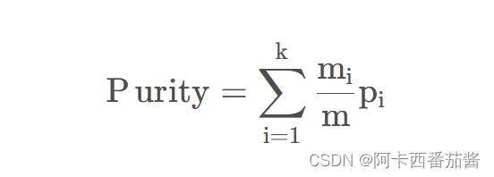
先给出Purity的计算公式:
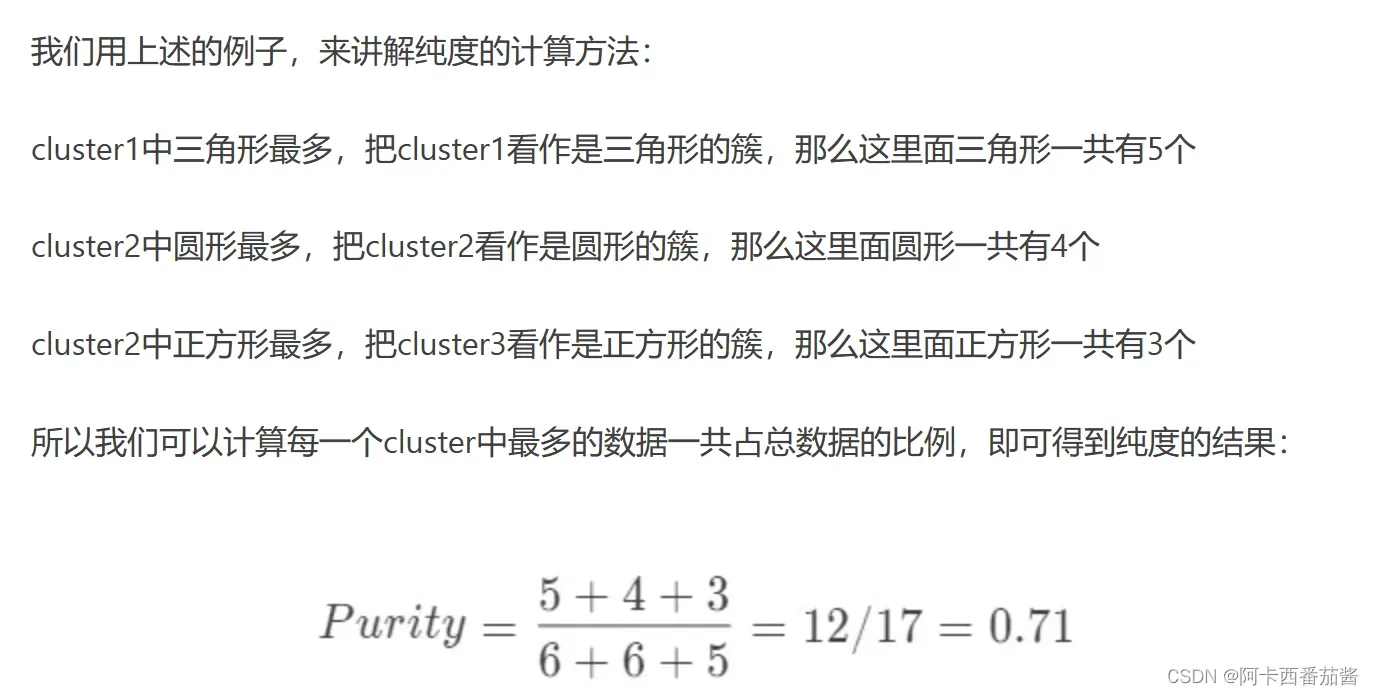
首先解释一下,为什么需要引入纯度计算,因为聚类中总是会出现此类与标签对应的类不一致,虽然他们表示的数字都是1,但是实质内容可能不一致。
用一个例子说明,例子借用了博客评价聚类的指标:纯度、兰德系数以及调整兰德系数 – 简书
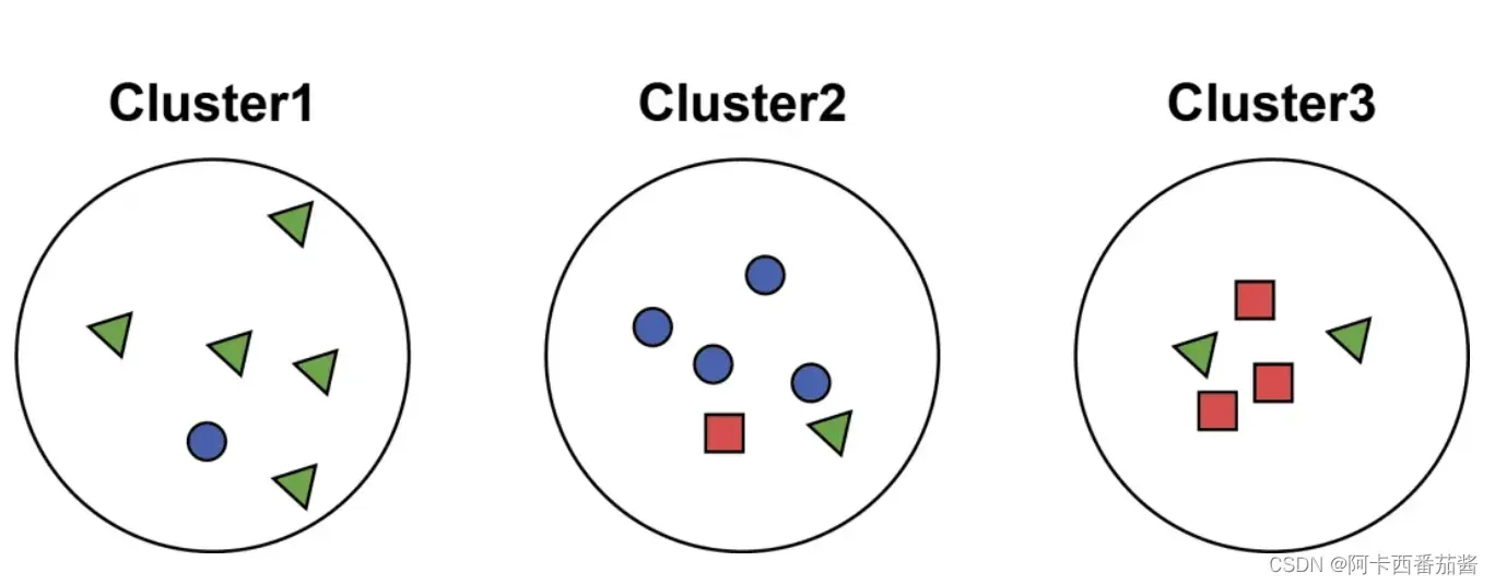
详细请见上述我附上的链接地址~
Python代码
def purity(labels_true, labels_pred):
    clusters = np.unique(labels_pred)
    labels_true = np.reshape(labels_true, (-1, 1))
    labels_pred = np.reshape(labels_pred, (-1, 1))
    count = []
    for c in clusters:
        idx = np.where(labels_pred == c)[0]
        labels_tmp = labels_true[idx, :].reshape(-1)
        count.append(np.bincount(labels_tmp).max())
    return np.sum(count) / labels_true.shape[0]
Matlab代码
function [purity] = Purity(labels_true, labels_pred)
clusters = unique(labels_pred);
labels_true = labels_true';
labels_pred = labels_pred';
labels_true = labels_true(:);
labels_pred = labels_pred(:);
count = [];

for c = 1:length(clusters)
	idx = find(labels_pred == c);
	temp = labels_true(idx);
	labels_tmp = reshape(temp,1,length(temp(:)));
	T=tabulate(labels_tmp);
	count = [count, max(T(:,2))];
end
purity = sum(count)/size(labels_true,1);
end
感谢Redmor提供的matlab代码~
1.2 ARI
原理解释
参考博客 调整兰德系数(Adjusted Rand index,ARI)的计算_的图表~
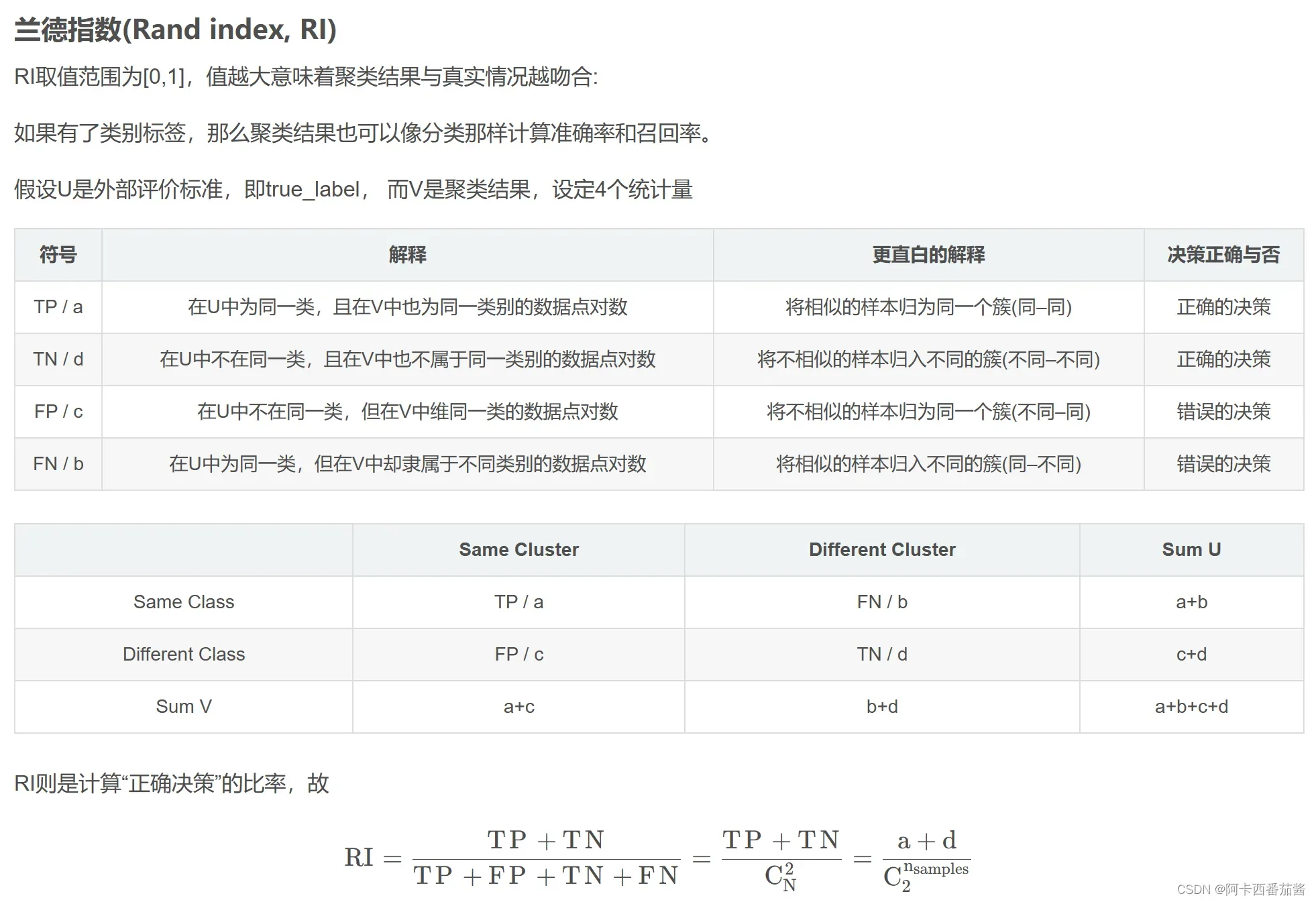
但是由于RI无法保证随机划分的聚类结果的RI值接近于0,所以现在主流科研工作者,使用的外部指标偏向于ARI,更加客观。
ARI的改进如下:
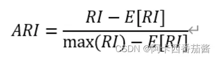
取值为[-1,1],绝对值越大效果越好~注意是绝对值噢。
Python 代码
def ARI(labels_true, labels_pred, beta=1.):
    from sklearn.metrics import adjusted_rand_score
    ari = adjusted_rand_score(labels_true, labels_pred)

    return ari
Matlab 代码
function ri = Eva_ARI(p1, p2, varargin)
%RAND_INDEX Computes the rand index between two partitions.
%   RAND_INDEX(p1, p2) computes the rand index between partitions p1 and
%   p2.
%
%   RAND_INDEX(p1, p2, 'adjusted'); computes the adjusted rand index
%   between partitions p1 and p2. The adjustment accounts for chance
%   correlation.

% Parse the input and throw errors
    adj = 0;
    if nargin == 0
    end
    if nargin > 3
        error('Too many input arguments');
    end
    if nargin == 3
        if strcmp(varargin{1}, 'adjusted')
            adj = 1;
        else
            error('%s is an unrecognized argument.', varargin{1});
        end
    end
    if length(p1)~=length(p2)
        error('Both partitions must contain the same number of points.');
    end

	% Preliminary computations and cleansing of the partitions
    N = length(p1);
    [~, ~, p1] = unique(p1);
    N1 = max(p1);
    [~, ~, p2] = unique(p2);
    N2 = max(p2);

    % Create the matching matrix
    for i=1:1:N1
        for j=1:1:N2
            G1 = find(p1==i);
            G2 = find(p2==j);
            n(i,j) = length(intersect(G1,G2));
        end
    end

    % If required, calculate the basic rand index
    if adj==0
        ss = sum(sum(n.^2));
        ss1 = sum(sum(n,1).^2);
        ss2 =sum(sum(n,2).^2);
        ri = (nchoosek2(N,2) + ss - 0.5*ss1 - 0.5*ss2)/nchoosek2(N,2);
    end


    % Otherwise, calculate the adjusted rand index
    if adj==1
        ssm = 0;
        sm1 = 0;
        sm2 = 0;
        for i=1:1:N1
            for j=1:1:N2
                ssm = ssm + nchoosek2(n(i,j),2);
            end
        end
        temp = sum(n,2);
        for i=1:1:N1
            sm1 = sm1 + nchoosek2(temp(i),2);
        end
        temp = sum(n,1);
        for i=1:1:N2
            sm2 = sm2 + nchoosek2(temp(i),2);
        end
        NN = ssm - sm1*sm2/nchoosek2(N,2);
        DD = (sm1 + sm2)/2 - sm1*sm2/nchoosek2(N,2);
        ri = NN/DD;
    end


    % Special definition of n choose k
    function c = nchoosek2(a,b)
        if a>1
            c = nchoosek(a,b);
        else
            c = 0;
        end
    end
end
hungarian函数可以直接去matlab中文社区获取噢或者后台私信我~
1.3 NMI
原理解释
MI, NMI, AMI(互信息,标准化互信息,调整互信息
大家可以参考这一篇博客,讲的很详细~
我就简单附上代码啦
Python 代码
def NMI_sklearn(predict, label):
    # return metrics.adjusted_mutual_info_score(predict, label)
    return metrics.normalized_mutual_info_score(predict, label)
Matlab代码
function z = Eva_NMI(x, y)
assert(numel(x) == numel(y));
n = numel(x);
x = reshape(x,1,n);
y = reshape(y,1,n);
l = min(min(x),min(y));
x = x-l+1;
y = y-l+1;
k = max(max(x),max(y));
idx = 1:n;
Mx = sparse(idx,x,1,n,k,n);
My = sparse(idx,y,1,n,k,n);
Pxy = nonzeros(Mx'*My/n);
Hxy = -dot(Pxy,log2(Pxy));
Px = nonzeros(mean(Mx,1));
Py = nonzeros(mean(My,1));
Hx = -dot(Px,log2(Px));
Hy = -dot(Py,log2(Py));
MI = Hx + Hy - Hxy;
z = sqrt((MI/Hx)*(MI/Hy));
z = max(0,z);
感谢开源社区~
1.4 ACC
精确度计算,有一点值得提醒,Python是直接与标签对比,没有进行Mapping步骤,适用于分类结果评估;matlab进行了Mapping步骤适用于聚类结果评估。
Python 代码
def AC(labels_true, labels_pre):
    acc = accuracy_score(labels_true, labels_pre)
    # acc = np.sum(labels_true==labels_pre) / np.size(labels_true)
    return acc
Matlab 代码
function [accuracy, ConMtx] = Eva_CA(dataCluster,dataLabel)

nData = length( dataLabel );
nC = max(dataLabel);
E = zeros( nC, nC );
for m = 1 : nData
    i1 = dataCluster( m );
    i2 = dataLabel( m );
    E( i1, i2 ) = E( i1, i2 ) + 1;
end
ConMtx=E';
E=-E;
[C,~]=hungarian(E);
nMatch=0;
for i=1:nC
    nMatch=nMatch-E(C(i),i);
end

accuracy = nMatch/nData;
以上外部指标均是目前科研工作者常用指标。
2 内部指标
与外部有效性指数相比,内部有效性指数评价的是数据分区的聚类结构,目的是衡量一个集群内聚类对象的比例,评估聚类对象的分布,而没有外部信息的支持。这里外部信息指原始数据的标签。
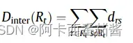
2.1 Internal and external validation measures (NCC)
原理解释
NCC 测量的是簇内距离和簇间距离的组合。簇内距离是指一个簇内物体之间的距离。作者将两个对象的 “群内协议”(Sintra)定义为两个对象之间的属性数量和群内距离之差。
距离的测量方法如下:
如果比较的所有属性值之间存在匹配,则drs=0,否则rs= N ⁄ 1,其中N是这两个对象之间在比较过程中发现的不匹配(mismatches)数量。
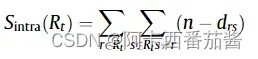
簇间距离 (Dinter),是不属于同一簇的两个对象(rands)之间的距离,也就是说,这个距离可以测量两个簇之间的距离。
Python 代码
def NCC(label, x):
    m = x.shape[0]
    n = x.shape[1]
    Y = np.zeros((m, m))
    for r in range(m):
        for s in range(m):
            if label[r] == label[s]:
                Y[r, s] = 1

    drs = np.zeros((m, m))
    for r in range(m):
        for s in range(m):
            for att in range(n):
                if x[r, att] != x[s, att]:
                    drs[r, s] += 1

    ncc = 0.0
    for r in range(m):
        for s in range(m):
            if r != s:
                ncc += (n - 2 * drs[r, s]) * Y[r, s] + drs[r, s]

    return ncc
Matlab 代码
function ncc = NCC_Y(Cluster_lable,x,n)

%%%Eq.(33)
% n is the number of attributes (categorical).
[m,~] = size(x);
Y = zeros(m,m);
for r = 1:m
    for s = 1:m
        if Cluster_lable(r) == Cluster_lable(s)
            Y(r,s) = 1;
        end
    end
end

drs = zeros(m,m);
for r = 1:m
    for s = 1:m
        for att = 1:n
            if x(r,att) ~= x(s,att)
                drs(r,s) = drs(r,s) + 1;
            end
        end
    end
end

ncc = 0;
for r = 1:m
    for s = 1:m
        if r~= s
            ncc = ncc + (n - 2*drs(r,s))*Y(r,s) + drs(r,s);
        end
    end
end
注释表示论文中的公式,参考文献附文末。
2.2 Entropy
原理解释
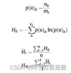
香农熵是在2001年提出的,用于计算数据集无序性的方法。应用于聚类的方法,如果一个簇数据尽可能地有序是否可以说明,更适合聚为一类呢?基于此,有学者Rˇezanková (2009)提出使用熵来计算一个集群中属性的无序性。
p(u)lt :u表示属性l中某一个可能的值,t表示一个簇,p(u)lt表示,在簇t中在l属性上拥有u值的频率。
Entropy值越小,代表聚类效果越好~
Python 代码
def Entropy(label, x):
    m = x.shape[0]
    n = x.shape[1]
    k = len(np.unique(label))
    # 每一个属性可能出现的值
    no_values = []
    for i in range(n):
        no_values.append(len(np.unique(x[:, i])))

    # cluster 成员数
    num_in_cluster = np.ones(k)
    for i in range(m):
        num_in_cluster[label[i]] += 1

    # p_u_lt
    P = []
    for t in range(k):
        # mt
        tp = np.where(label == t)[0]
        p_u_l = []
        for l in range(n):
            p_u_lt = []
            for u in range(no_values[l]):
                belong_lt = np.where(x[tp][:, l] == u)[0]
                p_u_lt.append(len(belong_lt) / len(tp))
            p_u_l.append(p_u_lt)
        P.append(p_u_l)

    # H
    H = np.zeros(k)
    for t in range(k):
        H_lt = np.zeros(n)
        for l in range(n):
            H_lt_u = np.zeros(no_values[l])
            for u in range(no_values[l]):
                if P[t][l][u] != 0:
                    H_lt_u[u] = - P[t][l][u] * np.log(P[t][l][u])
            H_lt[l] = np.sum(H_lt_u)
        H[t] = np.sum(H_lt) / n

    # H_R
    entropy_R = np.sum(H) / k

    return entropy_R
matlab代码
function entropy_R = Eva_Entropy(Cluster_lable,x,n)
% n is the number of attributes (categorical).

[m,~] = size(x);
t = length( unique( Cluster_lable ) );
R = cell(1,t);
value_lable = unique( Cluster_lable );
number_in_cluster = zeros(1,t);

for i = 1:m
    for j = 1:t
        if Cluster_lable(i) == value_lable(j)
            number_in_cluster(1,j) = number_in_cluster(1,j) + 1;
        end
    end
end

for i = 1:t
    R{i} = zeros(number_in_cluster(1,i),n);
end

%record cluster R
for i = 1:t
    count_x_in_rt = 1;
    for j = 1:m
        if Cluster_lable(j) == value_lable(i)
            for v = 1:n
                R{i}(count_x_in_rt,v) = x(j,v);
            end
            count_x_in_rt = count_x_in_rt + 1;
        end
    end
end

%number of attr
num_att = zeros(1,n);
for i = 1:n
    num_att(1,i) = length(unique(x(:,i)));
end

%value of attr
value_att = cell(1,n);
for i = 1:n
    value_att{i} = unique(x(:,i));
end

%probabilities,Eq.34
p_ult = cell(1,n);
for i = 1:n
    p_ult{i} = zeros(t,num_att(1,i));
end


for i = 1:n
    for j = 1:num_att(1,i)
        for k = 1:t
            nlt = 0;
            for mmt = 1:number_in_cluster(1,k)
                if value_att{i}(j) == R{k}(mmt,i)
                    nlt = nlt + 1;
                end
            end
            nlt = nlt / number_in_cluster(1,k);
            p_ult{i}(k,j) = nlt / number_in_cluster(1,k);
        end
    end
end


%Hlt,Eq.35
Hlt = zeros(t,n);
for i = 1:t
    for j = 1:n
        for v = 1:num_att(1,j)
            if p_ult{j}(i,v) ~= 0
                Hlt(i,j) = Hlt(i,j) - p_ult{j}(i,v)*log(p_ult{j}(i,v));
            end
        end
    end
end

%Eq.36
Ht = zeros(1,t);
for i = 1:t
    for j = 1:n
        Ht(1,i) = Ht(1,i) + Hlt(i,j);
    end
    Ht(1,i) = Ht(1,i)/n;
end

%Eq.37
entropy_R = 0;
for i = 1:t
    entropy_R = entropy_R + Ht(1,i);
end
entropy_R = entropy_R / t;
2.3 Compactness
原理解释
一个聚类’‘i’’的Compactness度量被定义为其元素之间的平均距离。这个平均值被称为簇的直径或Compactness。
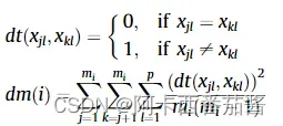
xjl 表示 对象 j 的第 l 个属性,同理xkl;
i表示第i个簇;
m表示数据集所有对象的和;
mi表示聚类i中对象和。
计算上述公式,得到直径,接下来就可以计算Compactness:
C表示簇的总和。
Python 代码
def compactness(label, x):
    m = x.shape[0]
    n = x.shape[1]
    k = len(np.unique(label))
    value_label = np.unique(label)

    number_in_cluster = np.zeros(k, int)
    for i in range(m):
        for j in range(k):
            if label[i] == value_label[j]:
                number_in_cluster[j] += 1

    R = np.zeros(k)
    for i in range(k):
        R[i] = np.zeros((number_in_cluster[i], n))

    for i in range(k):
        count_x_in_rt = 0
        for j in range(m):
            if label[j] == value_label[i]:
                for v in range(n):
                    R[i][count_x_in_rt, v] = x[j, v]
                count_x_in_rt += 1

    dm = np.zeros(k)
    for i in range(k):
        for j in range(number_in_cluster[i]):
            for h in range(j + 1, number_in_cluster[i]):
                for l in range(n):
                    # Eq.38
                    dt = 0
                    if R[i][j, l] != R[i][h, l]:
                        dt = 1
                    dm[i] += dt ** 2

        dm[i] = dm[i] / (number_in_cluster[i] * (number_in_cluster[i] - 1))

    Compactness = np.zeros(k)
    for i in range(k):
        Compactness[i] = dm[i] * (number_in_cluster[i] / m)
    Compactness = np.sum(Compactness)

    return Compactness
Matlab 代码
function  Compactness = CpS(Cluster_lable,x,n)
% n is the number of attributes (categorical).

[m,~] = size(x);
t = length( unique( Cluster_lable ) );
R = cell(1,t);
value_lable = unique( Cluster_lable );
number_in_cluster = zeros(1,t);

for i = 1:m
    for j = 1:t
        if Cluster_lable(i) == value_lable(j)
            number_in_cluster(1,j) = number_in_cluster(1,j) + 1;
        end
    end
end

for i = 1:t
    R{i} = zeros(number_in_cluster(1,i),n);
end

%record cluster R
for i = 1:t
    count_x_in_rt = 1;
    for j = 1:m
        if Cluster_lable(j) == value_lable(i)
            for v = 1:n
                R{i}(count_x_in_rt,v) = x(j,v);
            end
            count_x_in_rt = count_x_in_rt + 1;
        end
    end
end


%Eq.39
dm = zeros(1,t);
for i=1:t
    for j = 1:number_in_cluster(1,i)
        for k = j+1:number_in_cluster(1,i)
            for l = 1:n
                %Eq.38
                dt = 0;
                if R{i}(j,l) ~= R{i}(k,l)
                    dt = 1;
                end
                dm(1,i) = dm(1,i) + dt^2;
            end
        end
    end
    dm(1,i) = dm(1,i) / (number_in_cluster(1,i) * (number_in_cluster(1,i)-1));
end

Compactness = 0;
for i = 1:t
    Compactness = Compactness + dm(1,i)*(number_in_cluster(1,i)/m);
end
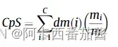
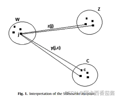
2.4 Silhouette Index
原理解释
轮廓系数我将引用论文中的一个图来解释
符号解释:
是被随机选择的一个object;
是j所属的簇;
w(j) 表示与对象j相同的,均来自同一聚类的所有对象,通俗化来说,即来自W的所有聚类对象之间相似度的平均值;
表示对象
和
之间的相似度;
,
是另外两个聚类。
使得 拥有最高的相似度,具体公式可以表示为:
- 第一种情况,当SHI(j) 接近1,表明该对象已经被 “紧紧地归类 “了。这种情况发生在集群W中的对象之间的平均相似度 w(j) 大于它们与集群 C 中的对象之间的相似度。换句话说,这意味着对象 j 不需要更换聚类方案了。
- 第二种情况,当SHI(j)值等于零,表明是两者均可的情况。这种情况发生在相似度 w(j )和 z(j) 所包含的数值几乎相等的情况下,因此,对象j在W和C中都会被紧密地聚在一起。
- 第三种情况,当SHI(j)值接近于-1的时候,表明对象 j 被 “糟糕地聚为一类”。当聚类中的对象之间的平均相似度w(j)小于该聚类和聚类C中的对象之间的相似度时,就会发生这种情况。一般来说,这意味着对象j在C群中的聚类效果比在W群中的效果更好。
Python 代码
from sklearn import metrics
# x means dataset;
metrics.silhouette_score(x,label)
有库就不用造轮子啦~
Matlab 代码
附图:
总结
聚类指标千千万,还得看你方法硬不硬,希望科研小白能继续坚持
整理不易,欢迎点赞关注支持~
文章出处登录后可见!