2.1 经验误差与过拟合
(1) 经验错误
| 基本术语 | 释义 |
|---|---|
| 错误率 | 分类错误的样本数占总样本数的比例 |
| 精度 | 精度=1-错误率 |
| 训练误差 | 在训练集上的误差 |
| 泛化误差 | 在新样本上的误差 |
(2) 过拟合
- 过拟合:模型的训练样本训练得很好,以至于训练样本本身的一些特征被认为是所有潜在样本都会具有的一般属性,这会导致泛化性能下降。
- 欠拟合:尚未学习到训练样本的一般属性
一般来说,欠拟合比较好解决,而过拟合无法彻底避免,只能尽量“缓解”(若可彻底避免过拟合,则说明可以获得最优解,即通过构造证明了“P=NP”)。
#mermaid-svg-JYotxW9CErq7fqq9 {font-family:”trebuchet ms”,verdana,arial,sans-serif;font-size:16px;fill:#333;}#mermaid-svg-JYotxW9CErq7fqq9 .error-icon{fill:#552222;}#mermaid-svg-JYotxW9CErq7fqq9 .error-text{fill:#552222;stroke:#552222;}#mermaid-svg-JYotxW9CErq7fqq9 .edge-thickness-normal{stroke-width:2px;}#mermaid-svg-JYotxW9CErq7fqq9 .edge-thickness-thick{stroke-width:3.5px;}#mermaid-svg-JYotxW9CErq7fqq9 .edge-pattern-solid{stroke-dasharray:0;}#mermaid-svg-JYotxW9CErq7fqq9 .edge-pattern-dashed{stroke-dasharray:3;}#mermaid-svg-JYotxW9CErq7fqq9 .edge-pattern-dotted{stroke-dasharray:2;}#mermaid-svg-JYotxW9CErq7fqq9 .marker{fill:#333333;stroke:#333333;}#mermaid-svg-JYotxW9CErq7fqq9 .marker.cross{stroke:#333333;}#mermaid-svg-JYotxW9CErq7fqq9 svg{font-family:”trebuchet ms”,verdana,arial,sans-serif;font-size:16px;}#mermaid-svg-JYotxW9CErq7fqq9 .label{font-family:”trebuchet ms”,verdana,arial,sans-serif;color:#333;}#mermaid-svg-JYotxW9CErq7fqq9 .cluster-label text{fill:#333;}#mermaid-svg-JYotxW9CErq7fqq9 .cluster-label span{color:#333;}#mermaid-svg-JYotxW9CErq7fqq9 .label text,#mermaid-svg-JYotxW9CErq7fqq9 span{fill:#333;color:#333;}#mermaid-svg-JYotxW9CErq7fqq9 .node rect,#mermaid-svg-JYotxW9CErq7fqq9 .node circle,#mermaid-svg-JYotxW9CErq7fqq9 .node ellipse,#mermaid-svg-JYotxW9CErq7fqq9 .node polygon,#mermaid-svg-JYotxW9CErq7fqq9 .node path{fill:#ECECFF;stroke:#9370DB;stroke-width:1px;}#mermaid-svg-JYotxW9CErq7fqq9 .node .label{text-align:center;}#mermaid-svg-JYotxW9CErq7fqq9 .node.clickable{cursor:pointer;}#mermaid-svg-JYotxW9CErq7fqq9 .arrowheadPath{fill:#333333;}#mermaid-svg-JYotxW9CErq7fqq9 .edgePath .path{stroke:#333333;stroke-width:2.0px;}#mermaid-svg-JYotxW9CErq7fqq9 .flowchart-link{stroke:#333333;fill:none;}#mermaid-svg-JYotxW9CErq7fqq9 .edgeLabel{background-color:#e8e8e8;text-align:center;}#mermaid-svg-JYotxW9CErq7fqq9 .edgeLabel rect{opacity:0.5;background-color:#e8e8e8;fill:#e8e8e8;}#mermaid-svg-JYotxW9CErq7fqq9 .cluster rect{fill:#ffffde;stroke:#aaaa33;stroke-width:1px;}#mermaid-svg-JYotxW9CErq7fqq9 .cluster text{fill:#333;}#mermaid-svg-JYotxW9CErq7fqq9 .cluster span{color:#333;}#mermaid-svg-JYotxW9CErq7fqq9 p.mermaidTooltip{position:absolute;text-align:center;max-width:200px;padding:2px;font-family:”trebuchet ms”,verdana,arial,sans-serif;font-size:12px;background:hsl(80, 100%, 96.2745098039%);border:1px solid #aaaa33;border-radius:2px;pointer-events:none;z-index:100;}#mermaid-svg-JYotxW9CErq7fqq9 :root{–mermaid-font-family:”trebuchet ms”,verdana,arial,sans-serif;} 无法避免 无法避免 无法避免 模型 欠拟合 决策树扩展分支 神经网络增加训练轮数 调参等其他方法 过拟合 神经网络提前终止训练 决策树剪枝 回归模型正则化
2.2 评估方法
为了衡量一个模型的泛化能力,需要使用“测试集”来测试模型对新样本的判别能力,测试集上的“测试误差”作为泛化误差的近似值.
测试集应遵循与训练集互斥的原则。
(1) 预订方法
- 直接将数据集
分成两个互斥的集合,需要考虑模型样本的平衡,必要时可以采用分层抽样的方法。
- 一次性放样法的结果不够可靠,需要多次随机划分,反复实验评价后取平均值。
- 通常选择2/3~4/5的样本作为训练集,剩余作为测试集。
#加载库
import numpy as np
import pandas as pd

#创建数据集
data=np.random.randint(100,size=[25,4])

#创建分割函数(此段代码为shenhuaifeng发布)
def split_train(data,test_ratio):
    shuffled_indices=np.random.permutation(len(data))
    test_set_size=int(len(data)*test_ratio)
    test_indices =shuffled_indices[:test_set_size]
    train_indices=shuffled_indices[test_set_size:]
    return data[train_indices],data[test_indices]

#切分训练集
train_data,test_data=split_train(data,0.2)
(2) 交叉验证方法
- 子集划分:交叉验证方法首先将数据集
大小相近的互斥子集,每个子集
通过分层抽样得到。
- 训练集挑选:每次用“
”个子集的并作为训练集,余下1个作为测试集。如是反复,
#加载库
from sklearn import datasets
from sklearn import metrics
from sklearn.model_selection import KFold,cross_val_score
from sklearn.pipeline import make_pipeline
from sklearn.linear_model import LogisticRegression
from sklearn.preprocessing import StandardScaler

# 加载手写数字的数据集
digits = datasets.load_digits()

# 创建特征矩阵
features = digits.data

#创建目标向量
target = digits.target

#创建标准化对象
standardizer =StandardScaler()

# 创建逻辑回归对象
logit=LogisticRegression()

#创建包含数据标准化和逻辑回归的流水线
pipeline = make_pipeline(standardizer,logit)

#创建k折交叉验证对象
kf = KFold(n_splits=10,shuffle=True,random_state=1)

#创建k折交叉验证
cv_results = cross_val_score(pipeline,features,target,cv=kf,scoring="accuracy")

# 计算得分
cv_results

#计算平均得分
cv_results.mean()
(3)自助法
bootstrap方法可以避免因划分区间而导致的训练集样本量减少的问题。
- 以bootstrap sampling为基础。给定包含
个样本的数据集
。
,极限约等于
。
- 以
作为测试集,这种测试结果称为“袋外估计”。
- 一般在数据量不足时使用
#载入包
import numpy as np

#创建数据集
data=np.random.randint(100,size=[25,4])

#定义自助法函数
def bootstrap_train(data):
    bootstrapping = []
    #自主法抽取样本号
    for i in range(len(data)):
        bootstrapping.append(np.floor(np.random.random()*len(data)))
    train_set = []
    #按样本号抽取样本保存为train_set
    for i in range(len(data)):
        train_set.append(data[int(bootstrapping[i])])
    #将train_set存储为np数组
    train_set = np.array(train_set)
    data_rows = data.view([('', data.dtype)] * data.shape[1])
    train_rows = train_set.view([('', train_set.dtype)] * train_set.shape[1])
    #data与train_data求差集
    test_data = (np.setdiff1d(data_rows, train_rows).view(data.dtype).reshape(-1, data.shape[1]))
    return train_set,test_data

train_data,test_data=bootstrap_train(data)
2.3 性能度量
回归任务中最常用的性能度量“均方误差”(MSE)。
(1) 错误率和准确率
对于样本集,分类错误率定义为:
准确度定义为:
#加载包
import numpy as np
from sklearn.metrics import accuracy_score

#准备数据
real = [0,0,1,0,1,0]
pred = [1,0,1,1,1,0]

#错误率
error_rate=1-accuracy_score(real,pred)

#精度
acc=accuracy_score(real,pred)
(二)查准率、查全率与F1
| 基本术语 | 英文 |
|---|---|
| 查准率 | precision |
| 查全率 | recall |
| 真正例 | true positive (TP) |
| 假正例 | false positive (FP) |
| 真反例 | true negative (TN) |
| 假反例 | false negative (FN) |
精度(准确度):
召回(召回):
- 检查和检查通常不兼容两者。
:
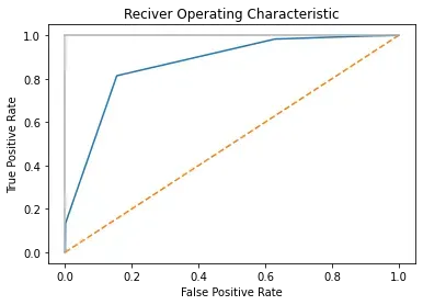
(三)ROC与AUC
ROC纵轴为真正例率(TPR),横轴为假正例率(FPR)。
AUC为ROC曲线下各部分面积之和。
#载入包
import numpy as np
import matplotlib.pyplot as plt

#读入TPR与FPR数据
true_positive_rate = np.array([0,0.133,0.814,0.983,0.997,1])
false_positive_rate = np.array([0,0.001,0.155,0.629,0.904,1])

#绘图
plt.title("Reciver Operating Characteristic")
plt.plot(false_positive_rate,true_positive_rate)
plt.plot([0,1],ls="--")
plt.plot([0,0],[1,0],c=".7"),plt.plot([1,1],c=".7")
plt.xlabel("False Positive Rate")
plt.ylabel("True Positive Rate")
plt.show()
文章出处登录后可见!