Experimental content
Coding MLP including one input layer, one hidden layer and one output layer. Additionally, output layer has two output neurons.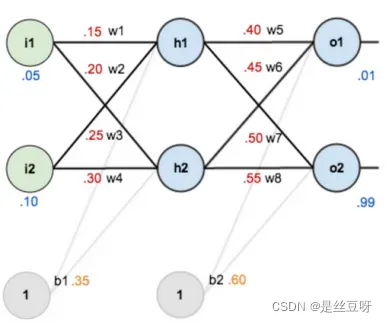
Experimental results
损失函数:均方误差(MSE)
激活函数:Sigmoid
- 代码:
# -*- coding: utf-8 -*-
# @Author : sido
# @Software: PyCharm
import numpy as np
import matplotlib.pyplot as plt
'''
损失函数:MSE
激活函数:Sigmoid
'''
def sigmoid(x): # 激活函数
return 1 / (1 + np.exp(-x))
# def MSE(y_pred, y):
# return ((y_pred - y) @ (y_pred - y).T) / len(y)
#
# def MAE(y_pred, y):
# return np.mean(abs(y_pred - y))
# ---------------------------- 参数初始化 -----------------------------
# np.random.seed(10)
x_input = np.array([0.05, 0.1, 1]) # shape(1, 3)
# w_input = np.array([[0.15, 0.20], [0.25, 0.30], [0.35, 0.35]]) # shape: (3, 2)
w_input = np.random.rand(3, 2)
# w_hidden = [[0.4, 0.45], [0.50, 0.55], [0.60, 0.60]] # shape: (3, 2)
w_hidden = np.random.rand(3, 2)
y = np.array([0.1, 0.99]) # shape: (1, 2)
a = 0.1 # 学习率
k = 1001 # 退出条件,迭代1001次
history_loss = [] # 记录训练过程中的损失
for i in range(k):
# ----------------------------- 前向传播 --------------------------
h_input = x_input @ w_input # shape: (1, 2)
h_output = np.hstack((sigmoid(h_input), 1)) # shape: (1, 3)
y_pred_input = h_output @ w_hidden # shape: (1, 2)
y_pred_output = sigmoid(y_pred_input) # shape: (1, 2)
temp = np.subtract(y, y_pred_output) # shape: (1, 2)
# ------------------------------ 计算梯度 ----------------------------
step1 = (- temp * y_pred_output * (1 - y_pred_output)).reshape(-1, 1) # shape: (2, 1)
step2 = (step1 @ np.expand_dims(h_output, axis = 0)).T # shape: (3, 2)
step3 = np.sum(step2[:2], axis=1).reshape(-1, 1) # shape: (2, 1)
step4 = step3 * (h_output[:2] * (1 - h_output[:2])).reshape(-1, 1) # shape: (2, 1)
step5 = (step4 @ np.expand_dims(x_input, axis = 0)).T
# ---------------------------- 更新参数 -----------------------------
w_hidden -= a * step2
w_input -= a * step5
# ---------------------------- 计算并记录损失 -------------------------
mae = (temp @ temp.T) / len(temp)
history_loss.append(mae)
if i % 100 == 0:
print(f"# 第{i}次 Loss: ", mae)
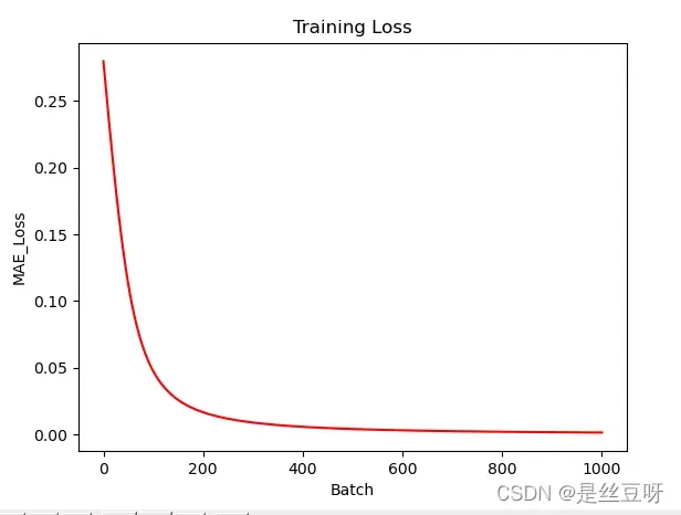
# -------------------------------- 绘制损失图像 --------------------------------
plt.title("Training Loss")
plt.xlabel("Batch")
plt.ylabel("MAE_Loss")
plt.plot([i for i in range(k)], history_loss, color='red')
plt.show()
- 代码输出:
# 第0次 Loss:  0.2797712656430154
# 第100次 Loss:  0.04744961852163526
# 第200次 Loss:  0.016702498979428736
# 第300次 Loss:  0.008973068224617735
# 第400次 Loss:  0.005788804421514717
# 第500次 Loss:  0.004132668628735767
# 第600次 Loss:  0.0031471498591124007
# 第700次 Loss:  0.0025065495053741916
# 第800次 Loss:  0.0020631623751121582
# 第900次 Loss:  0.0017414387680463237
# 第1000次 Loss:  0.0014992082423502138
- 绘制损失图像:
Experimental analysis
实验的难点主要在于计算梯度和反向传播
- 计算
时,不要加上绝对值
- 计算
sigmoid函数:
指导: - 实验过程中注意向量和矩阵形状的变化
可以采用 reshape, transpose 等来变换矩阵形状
不要混淆形状(2,)和(2, 1),两者是不同的,一个是一维的,一个是二维的
注:transpose不可以对一维向量进行转置
Conclusions
- 实验内容中给出的多层感知器的成功实现
- 成功实施反向传播以更新参数
- . 完成实验花费3~4个小时,主要时间花费在实现反向传播
- 首先是对反向传播的理解不够透彻,比较陌生
- 其次是对矩阵运算的生疏,不能熟练的运用Numpy库,对于每次计算的结果的向量、矩阵形状不能很好的把握,为了不出现由于矩阵形状不匹配而带来的矩阵运算错误,我将每次运算结果的形状标注在代码旁,这也花费了大量的时间。
- 虽然最终实现了实验,loss随着迭代次数收敛,但代码复用性较差,仅适用于实验内容中给出的多层感知器
- 报酬
对多层感知机有了更直观的理解与感受,在实践的过程中反复体验了梯度下降的过程,对损失在多层感知机中的传递以及参数的更新有了更深的理解,更熟悉矩阵的运算以及Numpy库使用。
文章出处登录后可见!
已经登录?立即刷新