03机器学习–梯度下降及python实现

内容

①概述

②梯度下降法的简单模拟

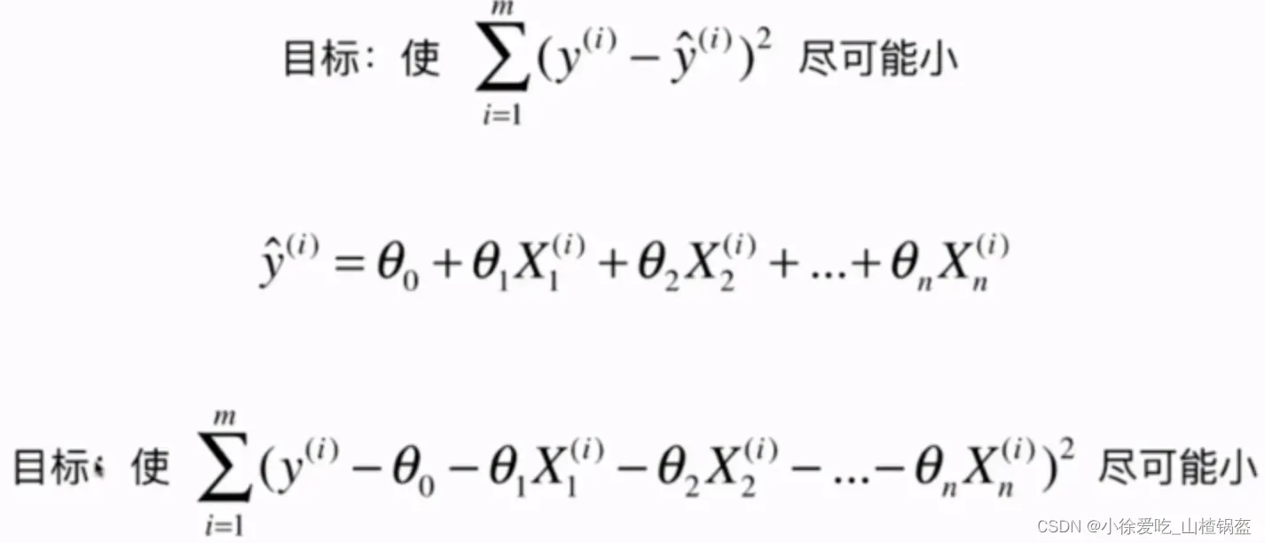
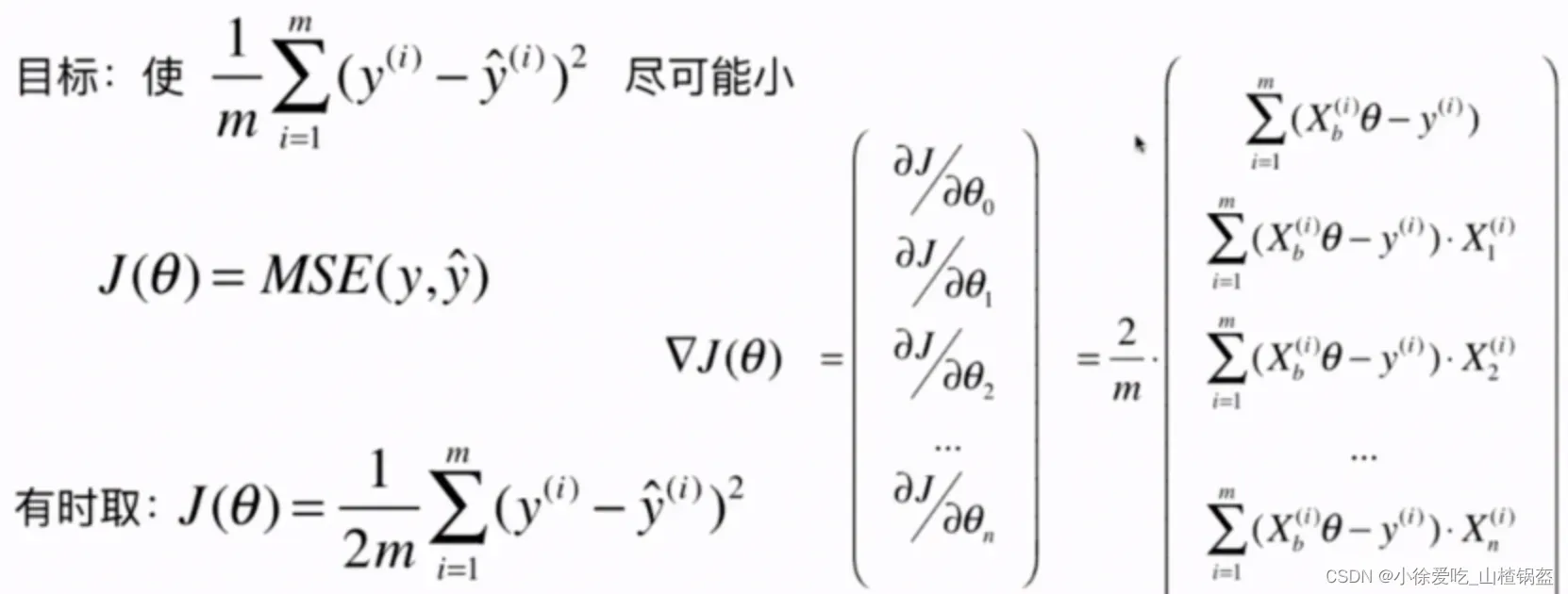
③ 在多元线性回归中使用梯度下降

④ 优化（梯度下降的向量化）

⑤ 数据归一化

⑥ 随机梯度下降

⑦scikit-learn中的随机梯度下降

⑧ 梯度调试

⑨总结

①概述

不是机器学习算法
是一种基于搜索的优化方法
作用：最小化损失函数
梯度上升：最大化效用函数

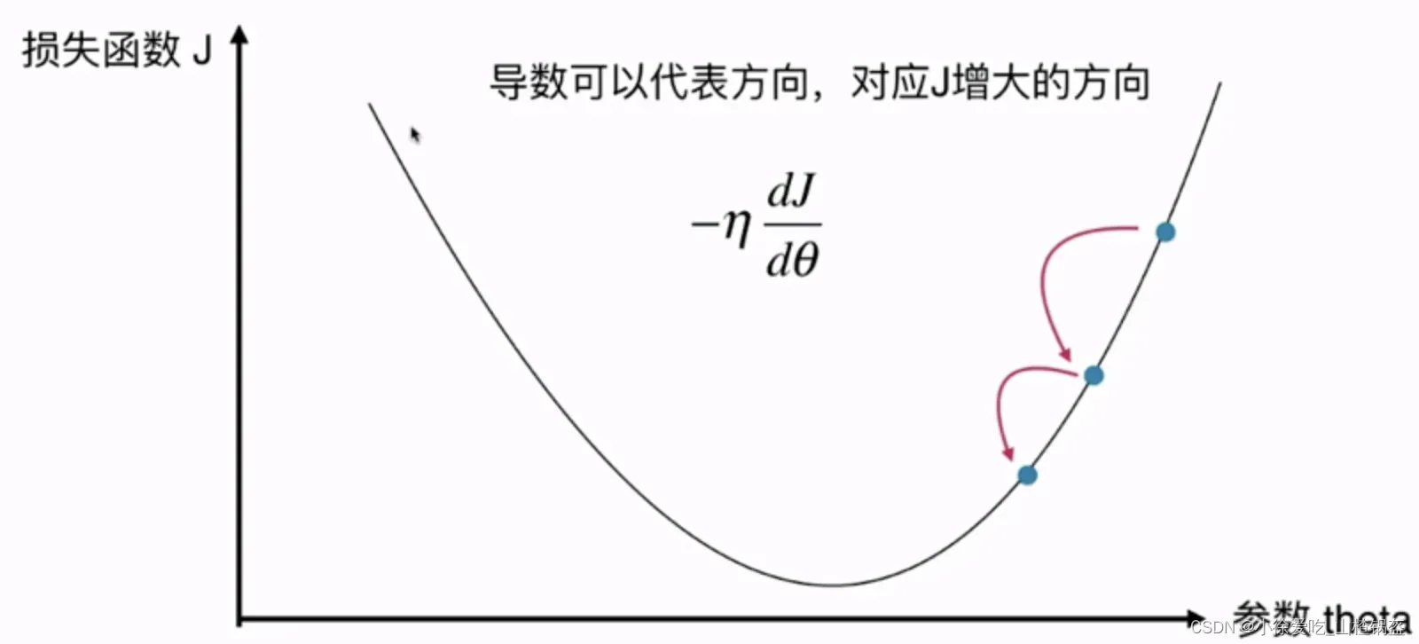
思路：由上图可知，在损失函数上的某一个点，希望经过变化到达损失函数最小值点，所以对损失函数求导，导数代表函数增大的方向，为了让函数变小，所以在导数前面增加负号，又因为需要逐步靠近最低点，所以在导数前面增加了步长 $\eta$ ，逐步靠近导数为0的位置。下降的速度就是由 $\eta$ 决定

$\eta$ 称为学习率（learning rate）
$\eta$ 的值影响获得最优解的速度
$\eta$ 的值不合适，甚至无法得到最优解。
$\eta$ 是梯度下降法的超参数

注意：并非所有函数都有唯一的极值点

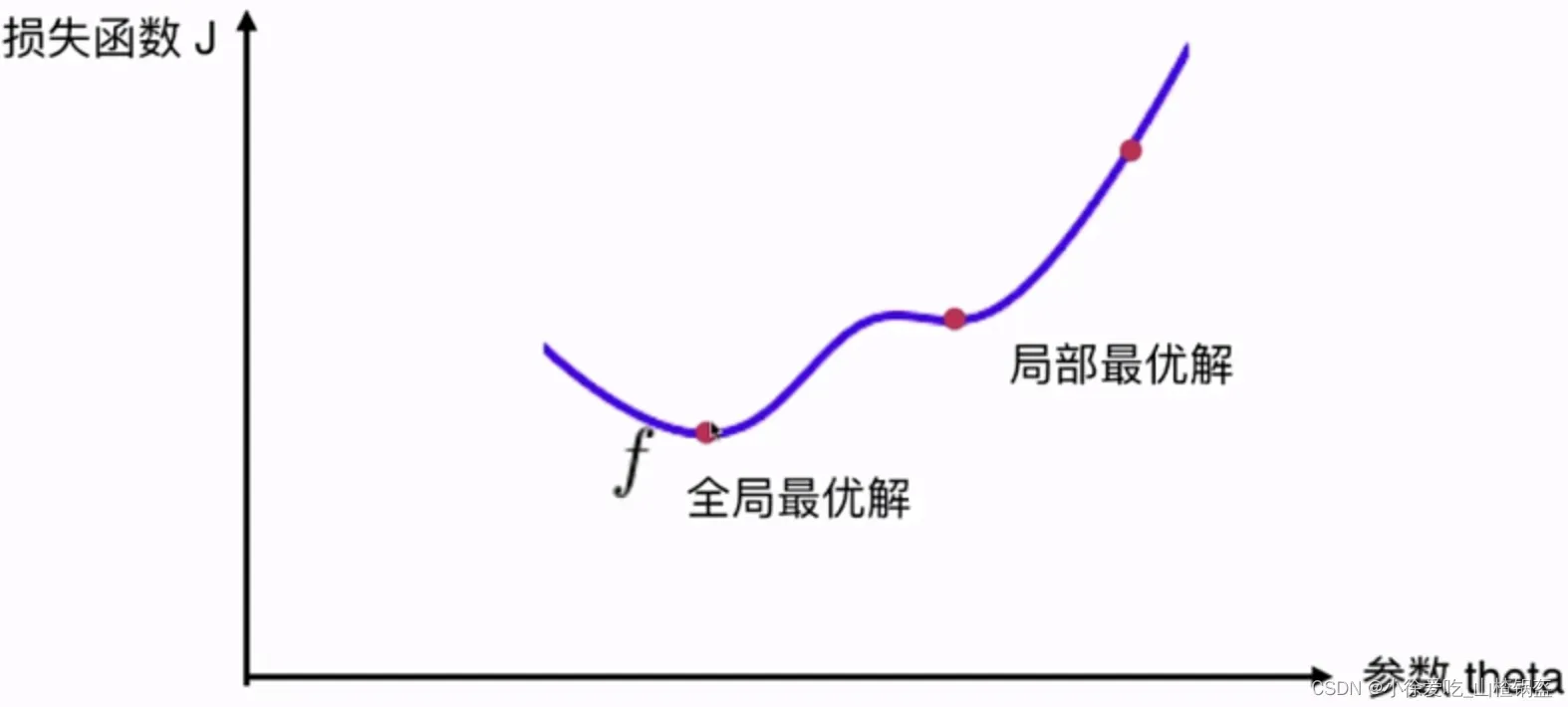
解决方案：

多次运行，随机化初始点
梯度下降的初始点也是一个超参数

②梯度下降法的简单模拟

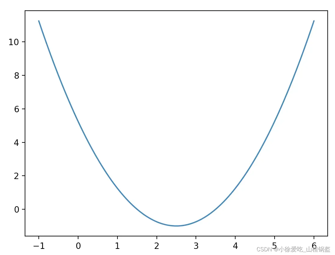
1）假设一个损失函数并绘制

import numpy as np
import matplotlib.pyplot as plt

# 随便画一个损失曲线
plot_x = np.linspace(-1, 6, 141)
plot_y = (plot_x - 2.5) ** 2 - 1
plt.plot(plot_x, plot_y)
plt.show()

输出结果：

2）实现梯度下降

import numpy as np
import matplotlib.pyplot as plt

# 随便画一个损失曲线
plot_x = np.linspace(-1, 6, 141)
plot_y = (plot_x - 2.5) ** 2 - 1
# plt.plot(plot_x, plot_y)
# plt.show()


def J(theta):  # 损失函数
    return (theta - 2.5) ** 2 - 1


def dJ(theta):  # 当前点的导数
    return 2 * (theta - 2.5)


# 梯度下降过程
theta = 0.0  # 一般以0为初始点
while True:
    gradient = dJ(theta)  # 求当前点对应的梯度（导数）
    last_theta = theta  # 学习前的theta
    eta = 0.1
    theta = theta - eta * gradient  # 参数值向导数负方向移动，eta为学习率，假设学习率为0.1

    epsilon = 1e-8  # 精度

    # 各种情况会导致最终导数不是刚好为0，如果每次学习过后，损失函数的减小值达到某一精度，我们就认为他学习结束（基本上到达最小值）
    if (abs(J(theta) - J(last_theta)) < epsilon):
        break

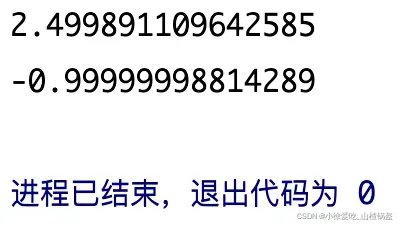
print(theta)  #  损失函数最小值横坐标
print(J(theta))  # 损失函数最小值

输出结果：

观看学习过程：

import numpy as np
import matplotlib.pyplot as plt

# 随便画一个损失曲线
plot_x = np.linspace(-1, 6, 141)
plot_y = (plot_x - 2.5) ** 2 - 1
# plt.plot(plot_x, plot_y)
# plt.show()


def J(theta):  # 损失函数
    return (theta - 2.5) ** 2 - 1


def dJ(theta):  # 当前点的导数
    return 2 * (theta - 2.5)


# 梯度下降过程
theta = 0.0  # 一般以0为初始点

theta_history = [theta]

while True:
    gradient = dJ(theta)  # 求当前点对应的梯度（导数）
    last_theta = theta  # 学习前的theta
    eta = 0.1
    theta = theta - eta * gradient  # 参数值向导数负方向移动，eta为学习率，假设学习率为0.1

    theta_history.append(theta)

    epsilon = 1e-8  # 精度

    # 各种情况会导致最终导数不是刚好为0，如果每次学习过后，损失函数的减小值达到某一精度，我们就认为他学习结束（基本上到达最小值）
    if (abs(J(theta) - J(last_theta)) < epsilon):
        break

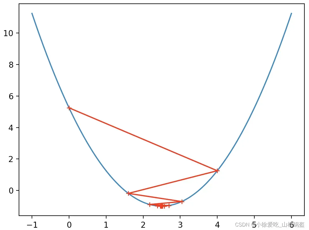
plt.plot(plot_x, J(plot_x))
plt.plot(np.array(theta_history), J(np.array(theta_history)), color="r", marker='+')
plt.show()

输出结果：

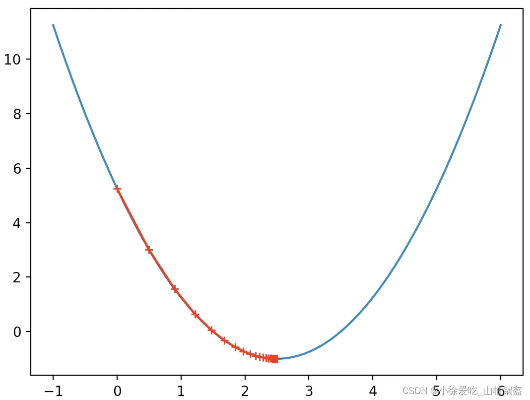
可以观察到，一开始运动的幅度比较大，因为一开始坡度比较陡，坡度变平缓，运动的幅度变小了。

3）改变一下学习率

import numpy as np
import matplotlib.pyplot as plt

# 随便画一个损失曲线
plot_x = np.linspace(-1, 6, 141)
plot_y = (plot_x - 2.5) ** 2 - 1

def J(theta):
    return (theta-2.5)**2 - 1.
def dJ(theta):
    return 2*(theta-2.5)

# 把上面的梯度下降函数封装起起来
def gradient_descent(initial_theta, eta, epsilon=1e-8):
    theta = initial_theta
    theta_history.append(initial_theta)

    while True:
        gradient = dJ(theta)
        last_theta = theta
        theta = theta - eta * gradient
        theta_history.append(theta)

        if (abs(J(theta) - J(last_theta)) < epsilon):
            break

# 绘制学痕迹
def plot_theta_history():
    plt.plot(plot_x, J(plot_x))
    plt.plot(np.array(theta_history), J(np.array(theta_history)), color="r", marker='+')
    plt.show()

eta = 0.01
theta_history = []
gradient_descent(0, eta)
plot_theta_history()

输出结果：

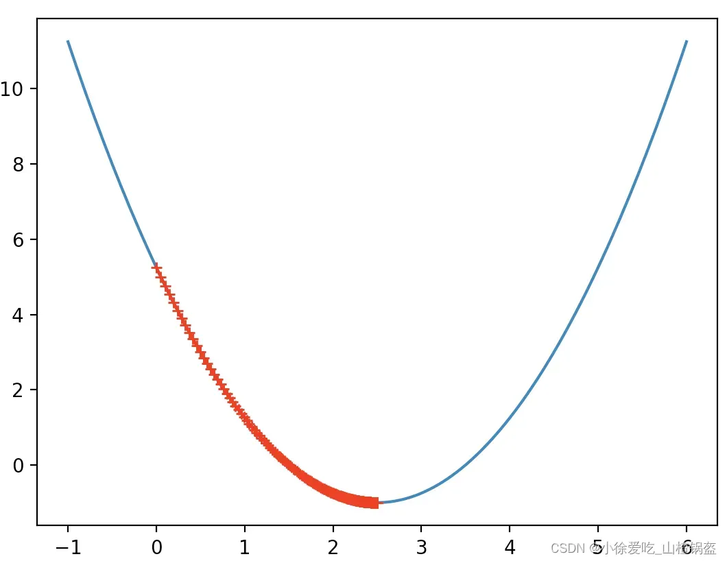
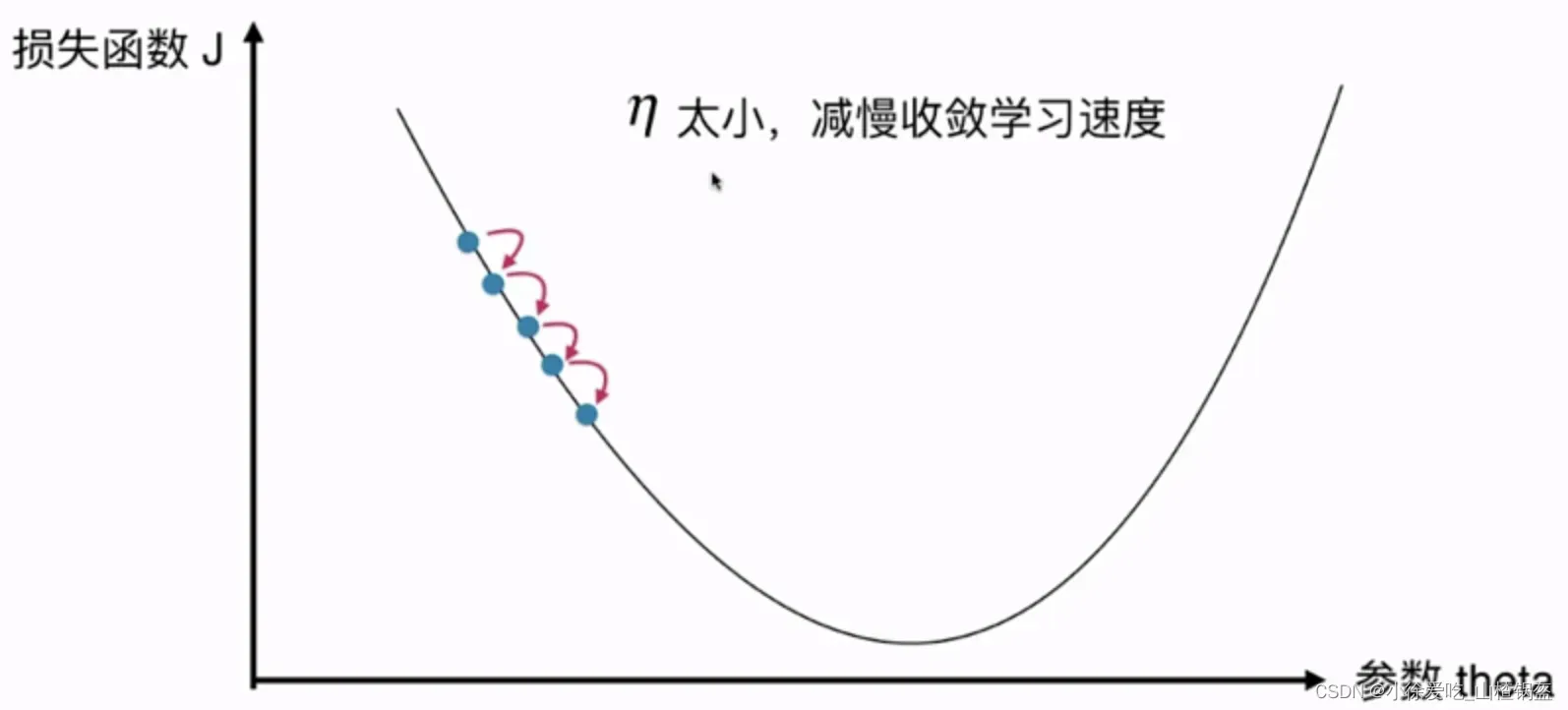
很明显学习的步数更多了，因为学习率（0.01）小了很多。

再改一下：学习率（0.8）后

输出结果：

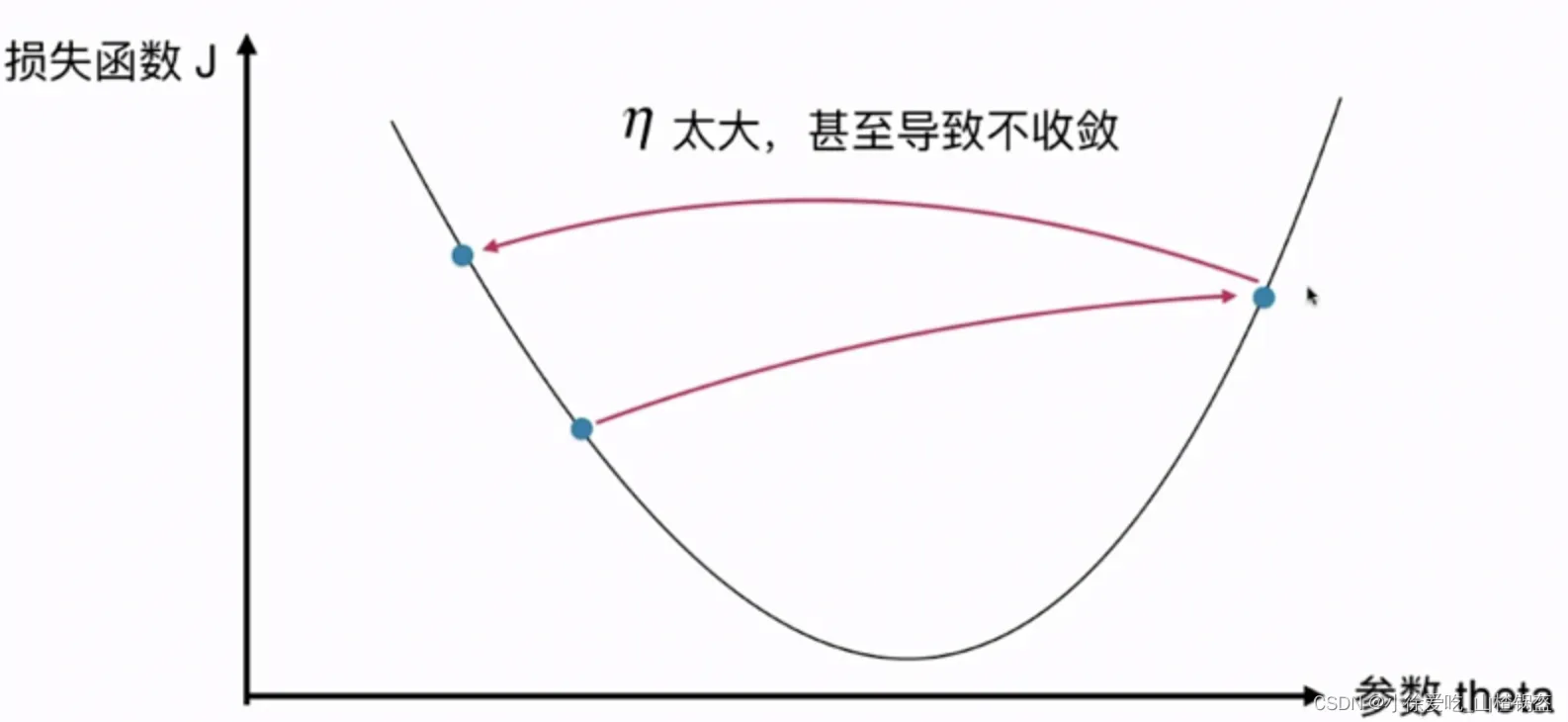
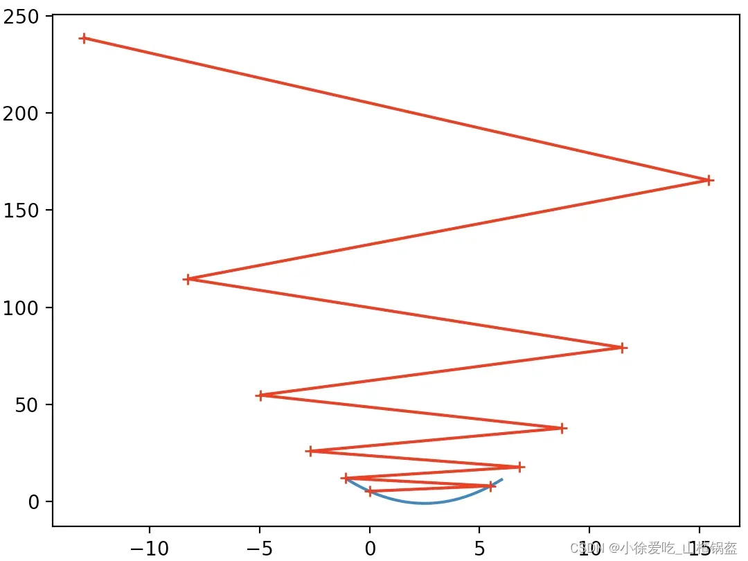
又改一下：学习率（1.1）后

输出结果：

你会发现一个错误，因为学习率太大，所以每次学习后，损失函数不是变小而是变大，而且一次次变大，最终的结果会很大。

限制循环次数（10次）观察一下：

import numpy as np
import matplotlib.pyplot as plt

# 随便画一个损失曲线
plot_x = np.linspace(-1, 6, 141)
plot_y = (plot_x - 2.5) ** 2 - 1

def J(theta):
    return (theta-2.5)**2 - 1.
def dJ(theta):
    return 2*(theta-2.5)

# 把上面的梯度下降函数封装起起来
def gradient_descent(initial_theta, eta, n_iters=1e4, epsilon=1e-8):
    theta = initial_theta
    i_iter = 0
    theta_history.append(initial_theta)

    while i_iter < n_iters:
        gradient = dJ(theta)
        last_theta = theta
        theta = theta - eta * gradient
        theta_history.append(theta)

        if (abs(J(theta) - J(last_theta)) < epsilon):
            break

        i_iter += 1

    return

# 绘制学痕迹
def plot_theta_history():
    plt.plot(plot_x, J(plot_x))
    plt.plot(np.array(theta_history), J(np.array(theta_history)), color="r", marker='+')
    plt.show()

eta = 1.1
theta_history = []
gradient_descent(0, eta, n_iters=10)
plot_theta_history()

输出结果：

③ 在多元线性回归中使用梯度下降

# coding=utf-8
import numpy as np
import matplotlib.pyplot as plt

# 编造一组数据
np.random.seed(666)  # 随机种子
x = 2 * np.random.random(size=100)  # 100个样本每个样本1个特征
y = x * 3 + 4 + np.random.normal(size=100)

X = x.reshape(-1, 1)

# 绘制样本
# plt.scatter(x, y)
# plt.show()


# 使用梯度下降法训练
def J(theta, X_b, y):  # 计算损失函数
    try:
        return np.sum((y - X_b.dot(theta)) ** 2) / len(X_b)
    except:
        return float('inf')


# 对损失函数求导
def dJ(theta, X_b, y):  # 导数 x_b是增加了第一列1的矩阵，上一节中有说明
    res = np.empty(len(theta))  # 开一个空间存最终结果
    res[0] = np.sum(X_b.dot(theta) - y)  # 第一项导数
    for i in range(1, len(theta)):  # 剩下项导数
        res[i] = (X_b.dot(theta) - y).dot(X_b[:, i])
    return res * 2 / len(X_b)


# 梯度下降的过程，上面写过的
def gradient_descent(X_b, y, initial_theta, eta, n_iters=1e4, epsilon=1e-8):
    theta = initial_theta
    cur_iter = 0

    while cur_iter < n_iters:
        gradient = dJ(theta, X_b, y)
        last_theta = theta
        theta = theta - eta * gradient
        if abs(J(theta, X_b, y) - J(last_theta, X_b, y)) < epsilon:
            break

        cur_iter += 1

    return theta


# 调用
X_b = np.hstack([np.ones((len(x), 1)), x.reshape(-1, 1)]) # 增加第一列
initial_theta = np.zeros(X_b.shape[1])
eta = 0.01

theta = gradient_descent(X_b, y, initial_theta, eta)
print(theta)  # 本例输出theta0和theta1分别对应截距和斜率

输出结果：

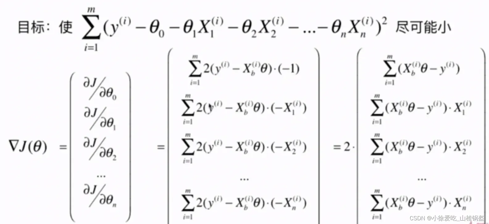
④ 优化（梯度下降的向量化）

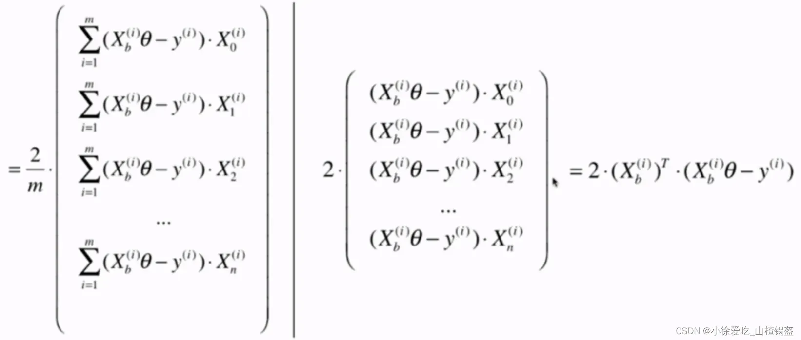
在上一部分梯度中每一项我们是用循环一个一个算出来的，这里对第0项进行变形：

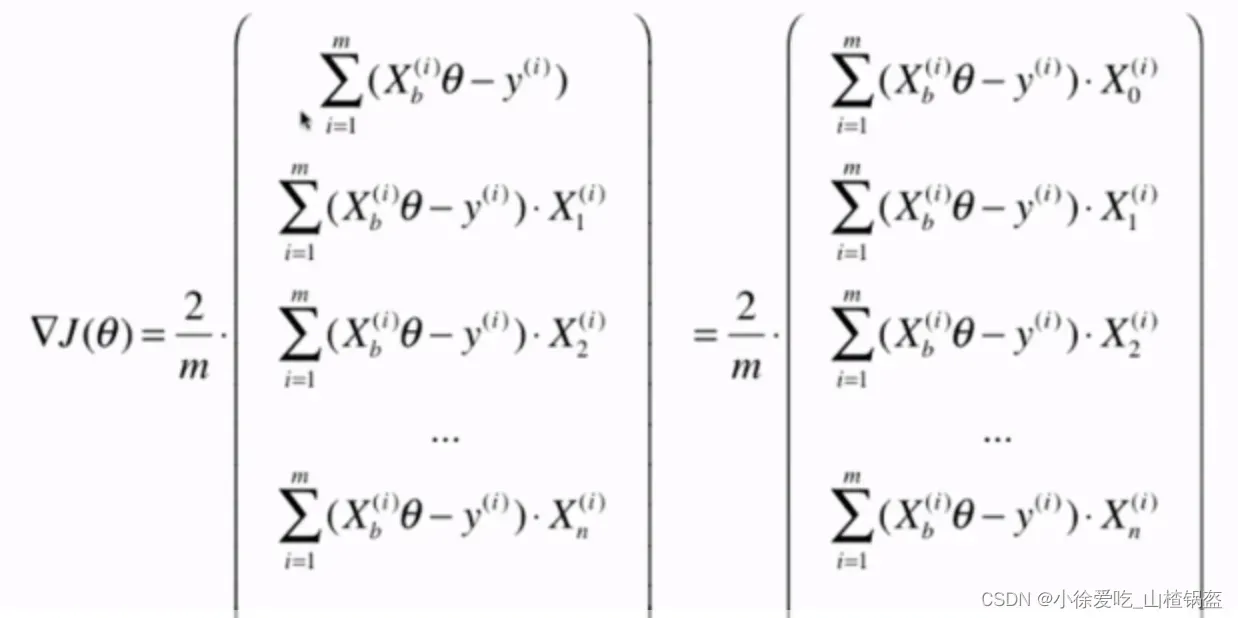
拆分为两个矩阵点积：（一个行向量）

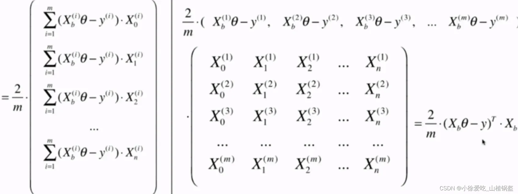
为了严谨起见，将其转置为流向量：（因为是列向量）

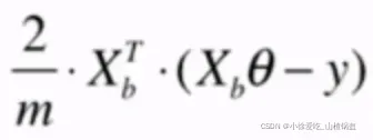
可以在原导函数的基础上进行修改。

# 把原来的dJ函数优化一下
def dJ(theta, X_b, y):
    return X_b.T.dot(X_b.dot(theta) - y) * 2 / len(X_b)

⑤ 数据归一化

解决不同数据维度的情况，因为不同的数据维度很可能会增加很多搜索时间，如第一章所述。

01机器学习–kNN分类学习笔记及python实现_小徐爱吃_山楂锅盔的博客-CSDN博客

⑥ 随机梯度下降

缺陷：上面提到的梯度下降法，每一次计算过程，都要对样本中对每一个x进行求导，属于批量梯度下降法。

优化：每次只对一个x进行求导，每次固定一个i

随机梯度下降法的搜索过程如下（不能保证每次方向都相同，存在一定的不可预测性）：

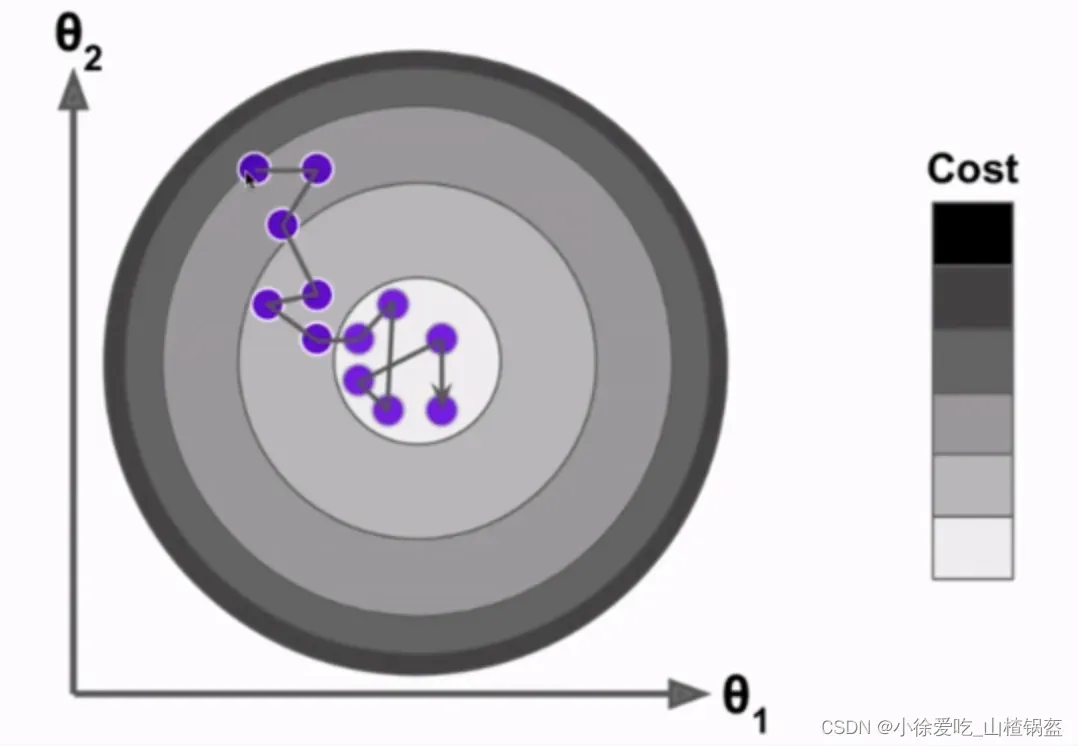
但是实验结果告诉我们他也是可行的，m非常大的话，宁愿损失一定的精度来换取时间，这时候随机梯度下降法的意义就体现出来了。

学习率的值变得非常重要。在实践中，希望学习率随着循环次数的增加而逐渐降低（个人理解越接近最低点越谨慎），如下：

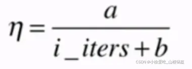
a，b就是随机梯度下降法中的超参数

import numpy as np
import matplotlib.pyplot as plt

m = 100000

x = np.random.normal(size=m)
X = x.reshape(-1, 1)
y = 4. * x + 3. + np.random.normal(0, 3, size=m)


def dJ_sgd(theta, X_b_i, y_i):  # 传的是X_b的某一行
    return 2 * X_b_i.T.dot(X_b_i.dot(theta) - y_i)


def sgd(X_b, y, initial_theta, n_iters): # 不用传学习率，这里不详细说明t的取值
    t0, t1 = 5, 50

    def learning_rate(t):  # 变化的学习率
        return t0 / (t + t1)

    theta = initial_theta
    for cur_iter in range(n_iters):
        rand_i = np.random.randint(len(X_b))  # 随机一个样本
        gradient = dJ_sgd(theta, X_b[rand_i], y[rand_i])
        theta = theta - learning_rate(cur_iter) * gradient

    return theta


X_b = np.hstack([np.ones((len(X), 1)), X])
initial_theta = np.zeros(X_b.shape[1])
theta = sgd(X_b, y, initial_theta, n_iters=m // 3)  # 这里人为的让循环次数为样本数的1/3
print(theta)

结果输出：

在这里使用的随机梯度比上面的批量梯度要节省许多时间，发现就算只循环了样本数的1/3页能够拟合到不错的效果，但是实际情况中不能人为的限制循环次数为1/3，这里只是想展示随机梯度的效果。

⑦scikit-learn中的随机梯度下降

只能求解线性模型

import numpy as np
from sklearn import datasets
# 前一章用过的房价数据集
boston = datasets.load_boston()
X = boston.data
y = boston.target
X = X[y < 50.0]
y = y[y < 50.0]
# 划分数据集
from sklearn.model_selection import train_test_split
X_train, X_test, y_train, y_test = train_test_split(X, y, test_size=0.2, random_state=666)
# 数据归一化
from sklearn.preprocessing import StandardScaler
standardScaler = StandardScaler()
standardScaler.fit(X_train)
X_train_standard = standardScaler.transform(X_train)
X_test_standard = standardScaler.transform(X_test)
# 梯度下降实现
from sklearn.linear_model import SGDRegressor
sgd_reg = SGDRegressor(n_iter_no_change=50) # 限定浏览次数，默认值5
sgd_reg.fit(X_train_standard, y_train)
print(sgd_reg.score(X_test_standard, y_test))

结果输出：

⑧ 梯度调试

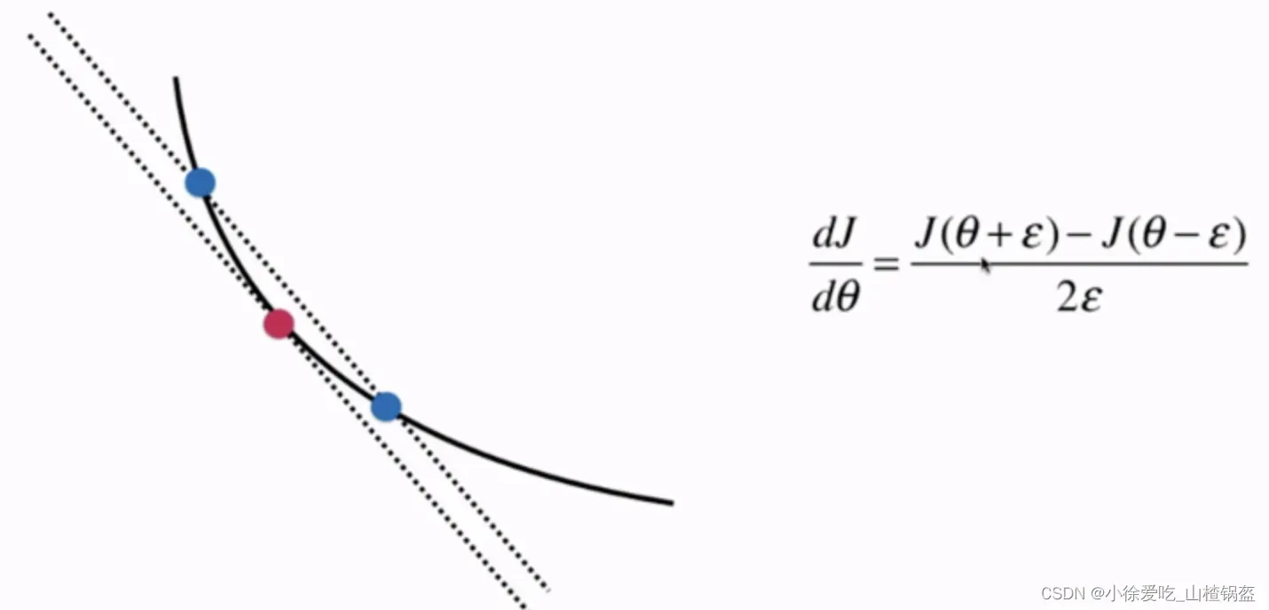
我怎样才能发现梯度是错误的？（衍生品可能被自己推错了）

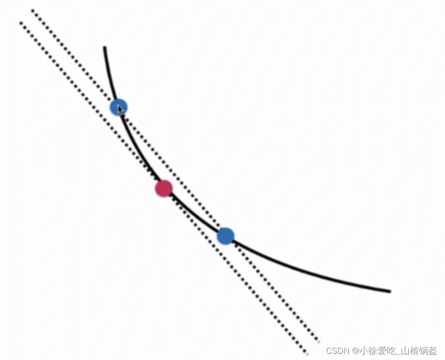
蓝点之间的距离越近，连接它们的直线的斜率与红点处切线的斜率大致相同

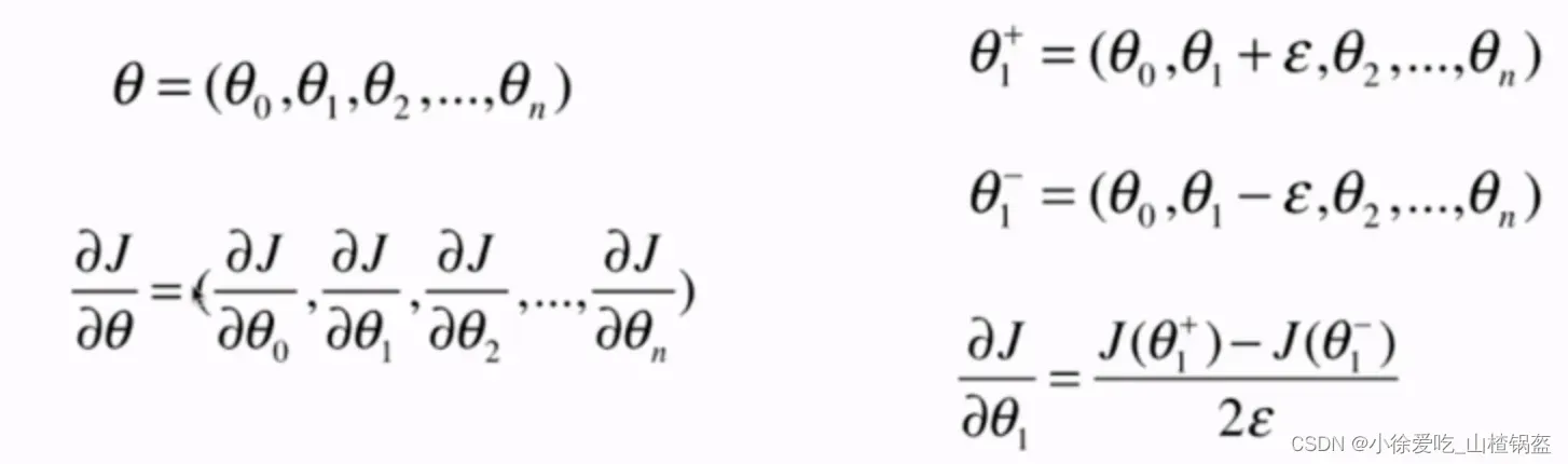
用于高尺寸

import numpy as np
import matplotlib.pyplot as plt

# 编一组数据
np.random.seed(666)
X = np.random.random(size=(1000, 10))
true_theta = np.arange(1, 12, dtype=float)
X_b = np.hstack([np.ones((len(X), 1)), X])
y = X_b.dot(true_theta) + np.random.normal(size=1000)

# 损失函数
def J(theta, X_b, y):
    try:
        return np.sum((y - X_b.dot(theta))**2) / len(X_b)
    except:
        return float('inf')

# 用数学推导的方式求导数
def dJ_math(theta, X_b, y):
    return X_b.T.dot(X_b.dot(theta) - y) * 2. / len(y)

# 用逼近的思想进行计算导数
def dJ_debug(theta, X_b, y, epsilon=0.01):
    res = np.empty(len(theta))
    for i in range(len(theta)): # 每一次求一个维度对应的值
        theta_1 = theta.copy()  # 原始的theta
        theta_1[i] += epsilon  # 第i个维度加一个邻域
        theta_2 = theta.copy()
        theta_2[i] -= epsilon  # 第i个维度减一个邻域
        res[i] = (J(theta_1, X_b, y) - J(theta_2, X_b, y)) / (2 * epsilon)  # 两点连线的斜率
    return res

# 批量梯度下降
def gradient_descent(dJ, X_b, y, initial_theta, eta, n_iters=1e4, epsilon=1e-8):
    theta = initial_theta
    cur_iter = 0

    while cur_iter < n_iters:
        gradient = dJ(theta, X_b, y)
        last_theta = theta
        theta = theta - eta * gradient
        if (abs(J(theta, X_b, y) - J(last_theta, X_b, y)) < epsilon):
            break

        cur_iter += 1

    return theta

X_b = np.hstack([np.ones((len(X), 1)), X])
initial_theta = np.zeros(X_b.shape[1])
eta = 0.01
theta = gradient_descent(dJ_debug, X_b, y, initial_theta, eta)
print(theta)
theta = gradient_descent(dJ_math, X_b, y, initial_theta, eta)
print(theta)

结果输出：

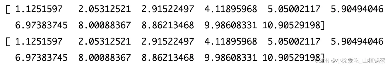
逼近的思路其实会跑的慢很多，但也是可行的。使用这种近似的思想，主要可以用来验证你开始推导的数学解是否正确。

⑨总结

批量梯度下降：求解缓慢，但稳定
随机梯度下降法：计算快，但不稳定，每次方向不确定
综合二者优缺点：小批量梯度下降法（每次看k个样本），这里不具体实现，只是在随机梯度的每次一个x改成k个x，多了一个超参数k。

一个关键概念——随机：跳出局部最优解，运行速度更快，如随机森林，随机搜索，后续介绍

梯度上升法：要找到一个目标函数的最大值，去掉学习率前面的负号。

文章出处登录后可见！

已经登录？立即刷新

03机器学习–梯度下降及python实现

①概述

②梯度下降法的简单模拟

③ 在多元线性回归中使用梯度下降

④ 优化（梯度下降的向量化）

⑤ 数据归一化

⑥ 随机梯度下降

⑦scikit-learn中的随机梯度下降

⑧ 梯度调试

⑨总结

相关推荐