Python 中的 NACA 翼型空气动力学简介
使用 Python 了解 NACA 4 系列机翼
本文旨在解释 NACA 翼型的基本特征,尤其适用于空气动力学入门的学生。首先讨论的是翼型几何背后的基本理论。然后,这些方程的 Python 实现计算相关的数值属性,以使用 Matplotlib 绘制 NACA 4 系列 2D 机翼轮廓。
Introduction
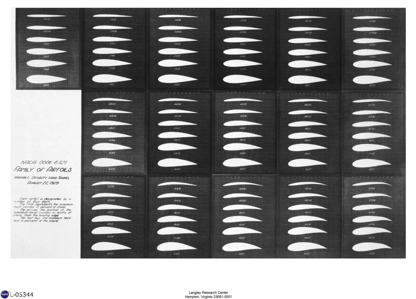
翼型是机翼的横截面。国家航空咨询委员会 (NACA) 开发并测试了一系列翼型,称为 NACA 翼型。图 1 显示了一系列此类示例机翼部分。[0]
四位数和五位数系列是初始空气动力学课程中最常学习的,但也有六位数模型。本文重点了解四位数系列,例如 NACA 4415 翼型。
翼型几何
图 2 是一个对称翼型样本,概述了关键几何参数。
- 前缘和后缘:分别是翼型的最前点和最后点
- 弦:连接翼型前缘和后缘的直线
- x:沿弦的水平距离,从前缘处的零开始
- y:相对于水平 x 轴的垂直高度
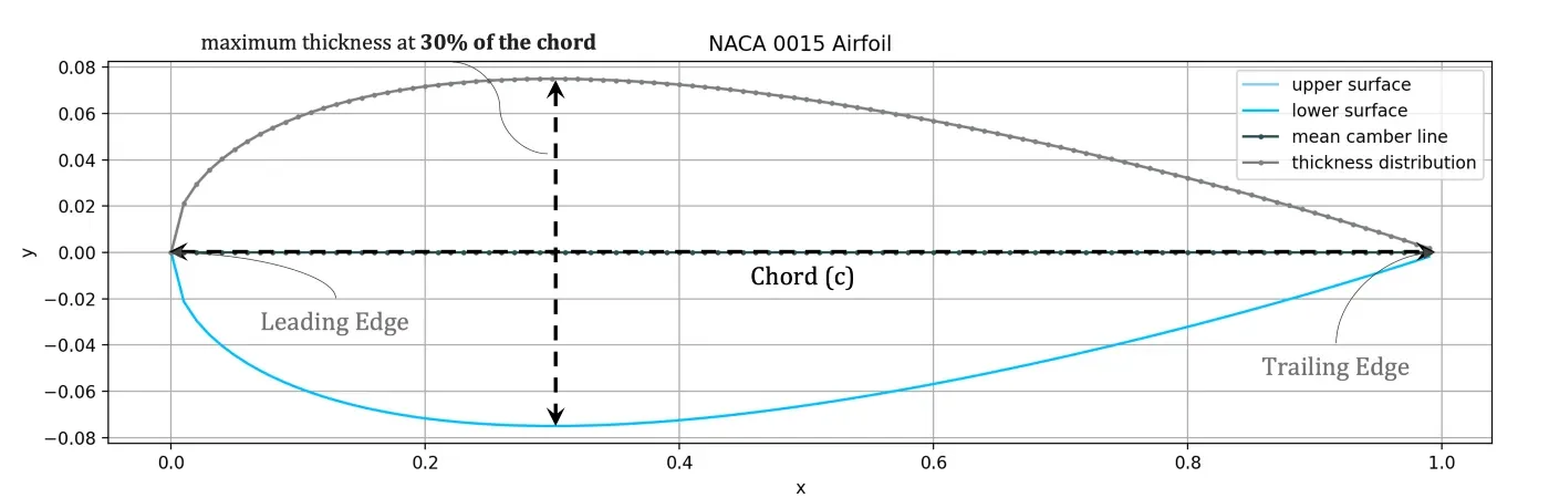
图 3 描绘了一个弧形翼型。弯度本质上类似于曲率。
- 中弧线:位于上下表面的中间,与几何中心线同义。
- 厚度 (t):高度沿翼型长度分布
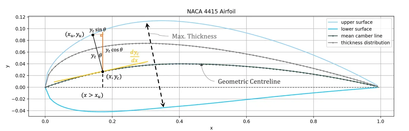
从图中可以明显看出,两个主要变量表示翼型表面的几何轮廓,弧度和厚度。
设计的一个关键方面是 4 系列机翼形状源自描述平均弧线和截面厚度分布的解析方程³。后来的系列,例如 6 系列,是使用复杂的理论方法推导出来的。
4 系列方程
NACA 4415 是 4 系列系列的示例成员。整数 4415 描述 2D 轮廓。
等式 1 对应于数字 1,以弦的百分比给出最大弯度 (m)。因此,4415 的最大外倾角为弦长的 4%。

数字 2 输入到等式 2 中,它提供了距前缘的最大外倾角 (p) 距离(以弦的十分之一为单位)。因此,4415 翼型的最大外倾点出现在沿弦长的 40% 处。

等式 3 使用数字 3 和 4;它们给出了翼型的最大厚度 (t) 占弦长的百分比。因此,4415 翼型厚度为弦长的 15%。

Gist 1 提供了 Python 代码,该代码定义了这三个函数,用于提取基于 NACA 四位数字的翼型特征。
对于对称翼型,前两位数字为零。即 0015 → m = 0,p = 0。
# ==============================================================
# naca four-digit series airfoil parameters


# maximum thickness (t) of the airfoil in percentage of chord
def max_wing_thickness(c, digit):
    """ calculate maximum wing thickness
    c: chord length
    digit: naca digits "34" of four series
    """
    return digit * (1 / 100) * c


# position of the maximum thickness (p) in tenths of chord
def distance_from_leading_edge_to_max_camber(c, digit):
    """ distance from leading edge to maxiumum wing thickness
    c: chord length
    digit: naca digit "2" of four series
    """
    return digit * (10 / 100) * c


# maximum camber (m) in percentage of the chord
def maximum_camber(c, digit):
    """ calculate maximum camber
    c: chord length
    digit: naca digit "1" of four series
    """
    return digit * (1 / 100) * c
两个方程根据 x 坐标是小于还是大于最大弧度 (p) 的位置来指定平均弧度线,如公式 4 所示。

重要的是要重申,所提出的方程纯粹是分析性的,由 NACA 通过研究和实验设计。
Gist 2 提供了公式 4 的 Python 实现。
def mean_camber_line_yc(m, p, X):
    """ mean camber line y-coordinates from x = 0 to x = p
    m: maximum camber in percentage of the chord
    p: position of the maximum camber in tenths of chord
    """
    return np.array([
        (m / np.power(p, 2)) * ((2 * p * x) - np.power(x, 2)) if x < p
        else (m / np.power(1 - p, 2)) * (1 - (2 * p) + (2 * p * x) - np.power(x, 2)) for x in X
    ])
yₜ 对应于厚度分布。高于 (+) 和低于 (-) 平均弧线的厚度值取决于公式 4。
x⁴ 系数根据后沿是打开还是关闭而变化。即,-0.1036 对应于封闭曲面,对于有限厚度的后缘,将 -0.1036 替换为 -0.1015。
yₜ 是在 Python 中使用 Gist 3 计算的。
def thickness_distribution(t, x):
    """ Calculate the thickness distribution above (+) and below (-) the mean camber line
    t: airfoil thickness
    x: coordinates along the length of the airfoil, from 0 to c
    return: yt thickness distribution
    """
    coeff = t / 0.2
    x1 = 0.2969 * np.sqrt(x)
    x2 = - 0.1260 * x
    x3 = - 0.3516 * np.power(x, 2)
    x4 = + 0.2843 * np.power(x, 3)
    # - 0.1015 coefficient for open trailing edge
    # - 0.1036 coefficient for closed trailing edge
    x5 = - 0.1036 * np.power(x, 4)
    return coeff * (x1 + x2 + x3 + x4 + x5)
垂直于平均弧线添加厚度值。因此,需要一个角度来指示加法的偏移量。
对平均弧线求导数得出曲线的切线斜率。将方程 4 对 x 进行微分得到方程 6。

使用 Gist 4 中的 Python 代码求平均弧线的导数。
def dyc_dx(m, p, X):
    """ derivative of mean camber line with respect to x
    m: maximum camber in percentage of the chord
    p: position of the maximum camber in tenths of chord
    """
    return np.array([
        (2 * m / np.power(p, 2)) * (p - x) if x < p
        else (2 * m / np.power(1 - p, 2)) * (p - x) for x in X
    ])
计算该导数的反正切得到角度 θ 以使厚度偏离垂直方向。参考图 3 来了解 θ 的作用在哪里。

最后,要计算上下翼型表面坐标,请使用公式 8-11,其中 θ 等于 MCL 在 x 处的导数的反正切,使用公式 7 确定。
Gist 6 提供了计算翼型上表面和下表面的最终 (x, y) 值的代码。

# ==============================================================
# final coordinates for the airfoil upper and lower surface

def x_upper_coordinates(x, yt, theta):
    """ final x coordinates for the airfoil upper surface """
    return x - yt * np.sin(theta)


def y_upper_coordinates(yc, yt, theta):
    """ final y coordinates for the airfoil upper surface """
    return yc + yt * np.cos(theta)


def x_lower_coordinates(x, yt, theta):
    """ final x coordinates for the airfoil lower surface """
    return x + yt * np.sin(theta)


def y_lower_coordinates(yc, yt, theta):
    """ final y coordinates for the airfoil lower surface """
    return yc - yt * np.cos(theta)


def theta(dyc, dx):
    return np.arctan(dyc / dx)
绘制结果
使用 (xᵤ, yᵤ) 和 (xₗ, yₗ) 的结果值绘制最终的机翼轮廓。图 4 描绘了使用 Matplotlib 绘制的 NACA 4415。
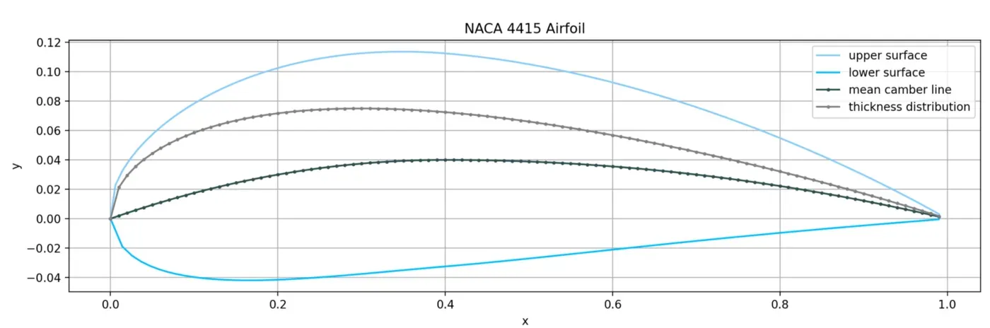
图 5 显示了另一个弧形 4 系列机翼样本,即 NACA 2412。直观地比较 4415 和 2412 的几何特性以查看差异,注意 y 轴刻度。
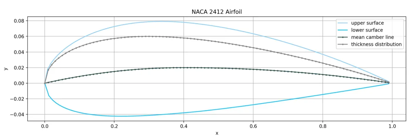
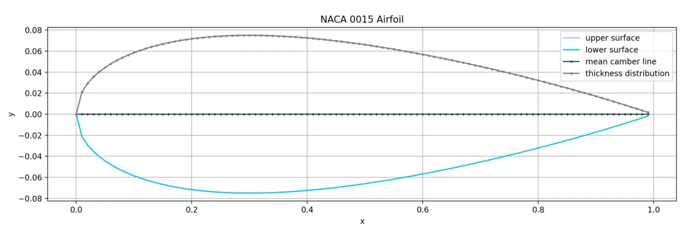
如前所述,这些解析表达式对对称翼型有效。
平均弧线和厚度分布都与弦完美对齐,在 0015 n 图 6 的结果图中可以清楚地看到。
Conclusion
每个方程都是通用的,可以用任意四个整数参数化,以可视化 4 系列 NACA 家族的任何成员。
本文概述了基本的翼型特性,并展示了一种实现几何表达式以绘制机翼 2D 表面轮廓的方法。
谢谢阅读。如果您对其他与空气动力学相关的文章感兴趣,请告诉我。
References
[1] 空气动力学基础。第六版。 John D. Anderson, Jr. 空气动力学策展人。国家航空航天博物馆。史密森学会。
[2] NACA 翼型——美国宇航局。最后更新:2017 年 8 月 7 日,编辑:鲍勃·艾伦
[3] NACA 翼型系列 (AA200_Course_Material) — 斯坦福
[4] 解释:NACA 4 位机翼 [飞机] — Josh The Engineer[0][1]
文章出处登录后可见!