1.什么是梯度下降法
机器学习领域的一个重要的方法,叫做梯度下降法。那么梯度下降法和我们之前讲的knn算法或者线性回归算法不同。梯度下降法本身不是一个机器学习的算法,他既不是在做监督学习,也不是在做非监督学习,他不能用于解决回归问题或者分类问题,梯度下降法是一种基于搜索的最优化的方法。它虽然也是人工智能领域的一个非常重要的方法,但是它的作用是用于优化一个目标函数。那么对于我们要最小化一个损失函数的话,相应的使用的就是梯度下降法。而如果我们要最大化一个效用函数的话,相应的就应该使用梯度上升法。
线性回归算法,最终我们要求解那个线性回归的模型。本质其实就是要最小化一个损失函数,我们在上一张直接计算出了最小化这个函数对应的参数它的数学解,但是我们后面就会看到。很多机器学习的模型是求不到这样的数学解的,那么基于这样的模型,我们就需要使用一种基于搜索的策略来找到这个最有解。那么梯度下降法就是在机器学习领域最小化损失函数的一个最为常用的方法。总体而言,在机器学习领域,熟练的掌握梯度法来求一个目标函数的最优值。是非常重要的一个事情。
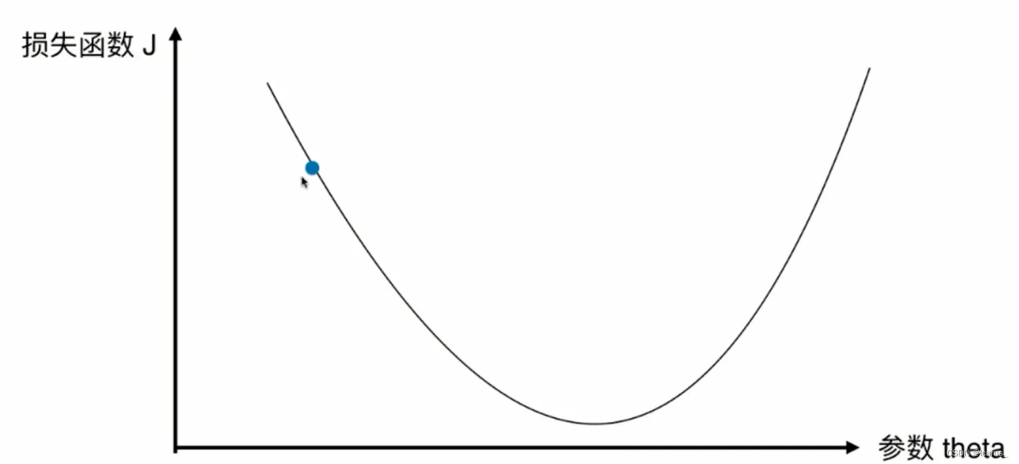
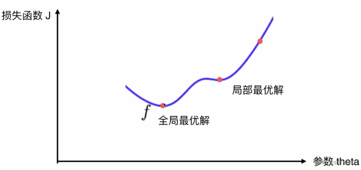
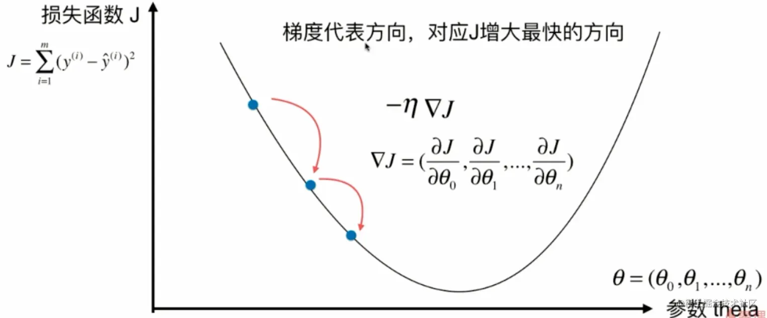
一个二维坐标平面不是描述特征平面,不是描述每一个特征点相对应的那个输出标记的值是多少。它描述的是,当我们定义了一个损失函数以后,这个y轴就是损失函数J它的取值,那么,相应的,如果我们取不同的参数。这个x轴代表参数,每取一个参数对应我们的损失函数J就会取到一个值。那么我们的这个损失函数J应该有一个最小值,对于我们最小化一个损失函数,这个过程来说相当于是在这样的一个坐标系中寻找合适的点参数。使得我们的这个损失函数J取得最小值,当然了,现在我是在二维平面上,所以,相当于我们的参数只有一个,我们使用这种可视化的方式帮助大家来理解什么是梯度下降法。
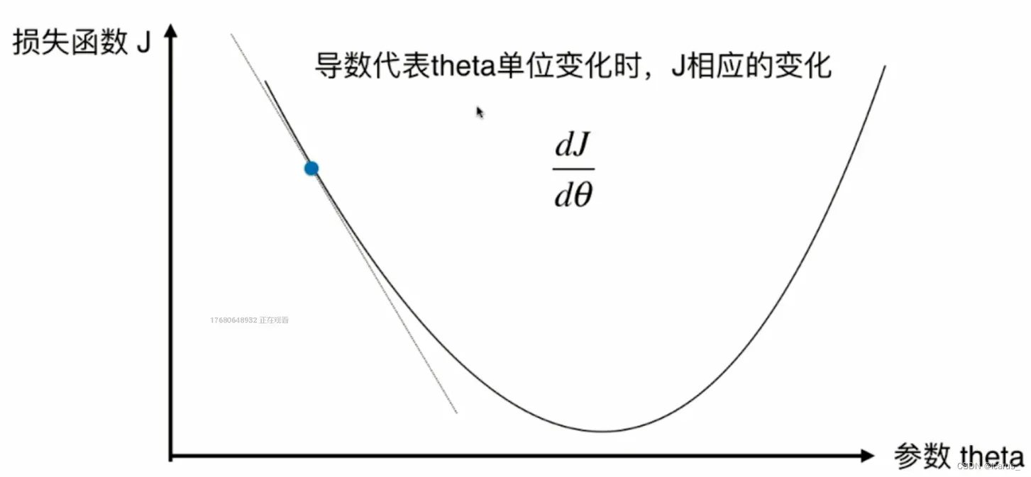
那么下面我们来看一下这个图。对于这个损失函数J来说,我每取一个值,相应的,它就有一个损失函数J,如果这一点它的倒数不为零的话,那么这一点肯定不在一个极值点上。


2.模拟实现梯度下降法
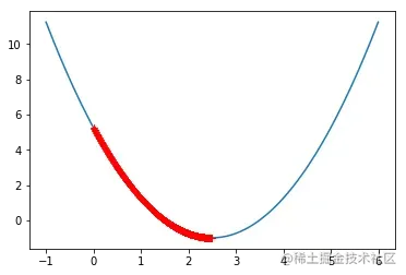
为了模拟这个梯度下降法呢,在这里,首先我们来确认一下我们的损失函数取什么,那么由于我们的这个损失函数是一个曲线,我们先把这个曲线来画出来。所以我在x轴上,从负1-6在这个范围来划一下我们的这个损失曲线。那么,为了绘制的这个曲线平滑呢,我相应的在这里面等间距的140个点
import numpy as np
import matplotlib.pyplot as plt

plot_x = np.linspace(-1., 6., 141)
plot_y = (plot_x-2.5)**2 - 1.
plt.plot(plot_x, plot_y)
plt.show()
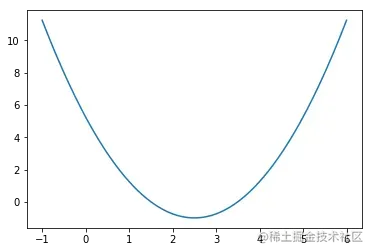
就以这根曲线为例。我们假设它就是我们的损失函数,我们希望使用梯度下降法找到这样一个曲线所对应的那个最小值在什么位置。要实现我们的梯度下降法,首先非常重要的,每一次我都要计算这个损失函数对应的导数。
epsilon = 1e-8
eta = 0.1
def J(theta):
return (theta-2.5)**2 - 1.
def dJ(theta):
return 2*(theta-2.5)
theta = 0.0
while True:
gradient = dJ(theta)
last_theta = theta
theta = theta - eta * gradient
if(abs(J(theta) - J(last_theta)) < epsilon):
break
print(theta)
print(J(theta))
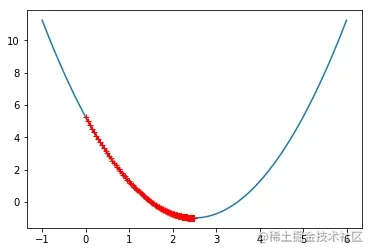
theta = 0.0
theta_history = [theta]
while True:
gradient = dJ(theta)
last_theta = theta
theta = theta - eta * gradient
theta_history.append(theta)
if(abs(J(theta) - J(last_theta)) < epsilon):
break
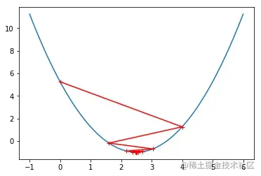
plt.plot(plot_x, J(plot_x))
plt.plot(np.array(theta_history), J(np.array(theta_history)), color="r", marker='+')
plt.show()

theta_history = []

def gradient_descent(initial_theta, eta, epsilon=1e-8):
    theta = initial_theta
    theta_history.append(initial_theta)

    while True:
        gradient = dJ(theta)
        last_theta = theta
        theta = theta - eta * gradient
        theta_history.append(theta)

        if(abs(J(theta) - J(last_theta)) < epsilon):
            break

def plot_theta_history():
    plt.plot(plot_x, J(plot_x))
    plt.plot(np.array(theta_history), J(np.array(theta_history)), color="r", marker='+')
    plt.show()

eta = 0.01
theta_history = []
gradient_descent(0, eta)
plot_theta_history()
eta = 0.001
theta_history = []
gradient_descent(0, eta)
plot_theta_history()
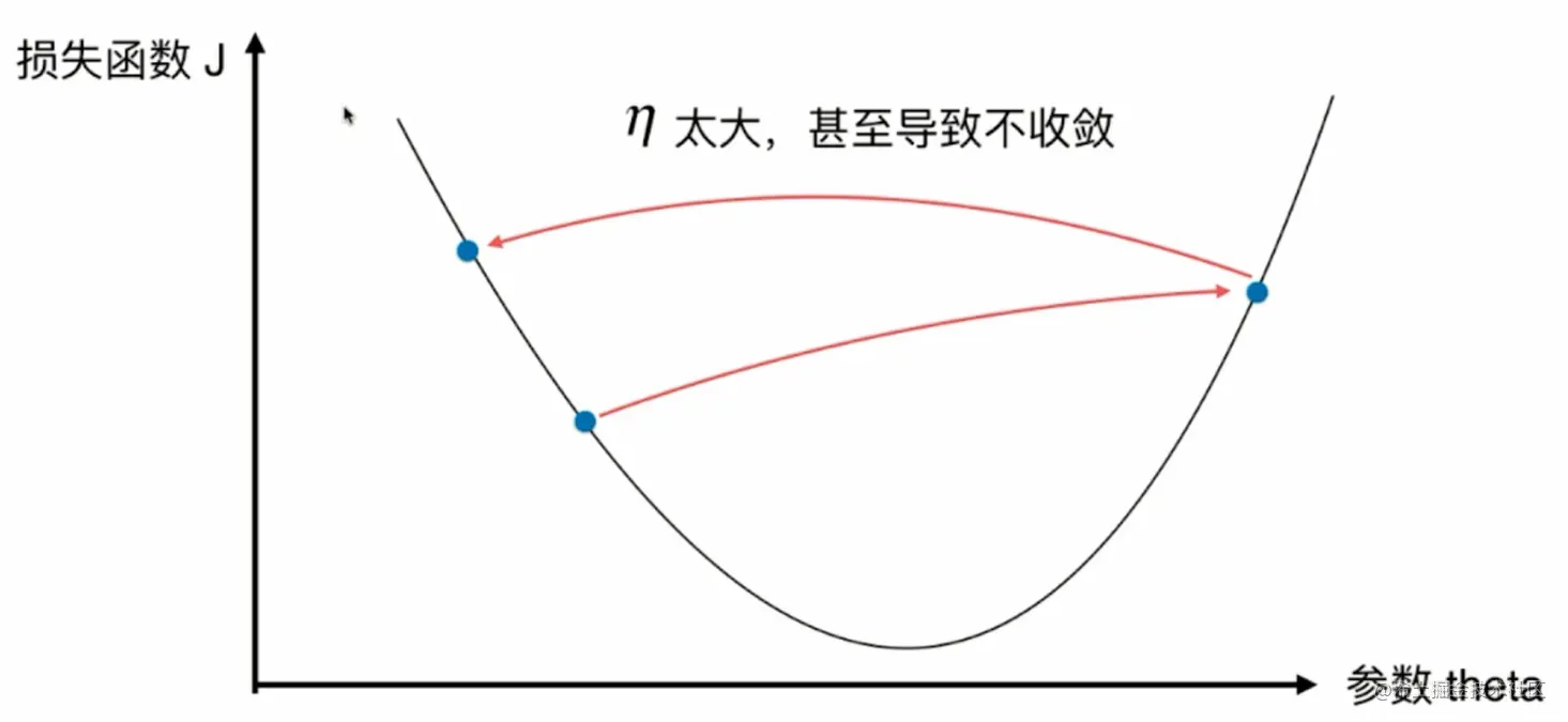
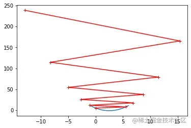
eta = 0.8
theta_history = []
gradient_descent(0, eta)
plot_theta_history()
def J(theta):
    try:
        return (theta-2.5)**2 - 1.
    except:
        return float('inf')

def gradient_descent(initial_theta, eta, n_iters = 1e4, epsilon=1e-8):

    theta = initial_theta
    i_iter = 0
    theta_history.append(initial_theta)

    while i_iter < n_iters:
        gradient = dJ(theta)
        last_theta = theta
        theta = theta - eta * gradient
        theta_history.append(theta)

        if(abs(J(theta) - J(last_theta)) < epsilon):
            break

        i_iter += 1

    return

eta = 1.1
theta_history = []
gradient_descent(0, eta, n_iters=10)
plot_theta_history()
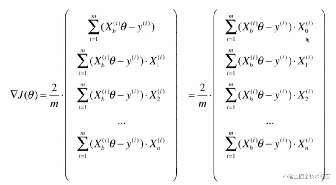
3.线性回归中的梯度下降法
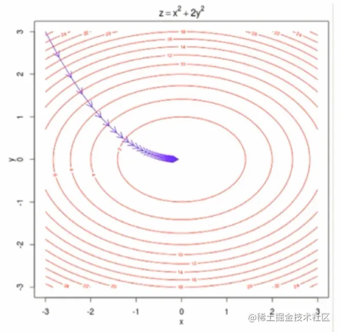
这个图呢是对一个有两个参数的梯度下降法进行的一个可视化,这一圈一圈的其实代表的是等高线,也就是说,代表的是损失函数J的取值。越外面的圈相应的J的取值越大。里面的圈,相应的J取值越小,那么在这个图的中心的位置达到这的最小值。当我们有多个参数的时候,在每一点的位置,我们向这取值更小的方向前进,其实有非常多的选择。但是,此时梯度那个方向相应的是下降最快的那个方向。
4.实现线性回归中的梯度下降法
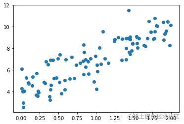
import numpy as np
import matplotlib.pyplot as plt

np.random.seed(666)
x = 2 * np.random.random(size=100)
y = x * 3. + 4. + np.random.normal(size=100)
X = x.reshape(-1, 1)
plt.scatter(x, y)
plt.show()
使用梯度下降法训练
def J(theta, X_b, y):
    try:
        return np.sum((y - X_b.dot(theta))**2) / len(X_b)
    except:
        return float('inf')

def dJ(theta, X_b, y):
    res = np.empty(len(theta))
    res[0] = np.sum(X_b.dot(theta) - y)
    for i in range(1, len(theta)):
        res[i] = (X_b.dot(theta) - y).dot(X_b[:,i])
    return res * 2 / len(X_b)

def gradient_descent(X_b, y, initial_theta, eta, n_iters = 1e4, epsilon=1e-8):

    theta = initial_theta
    cur_iter = 0

    while cur_iter < n_iters:
        gradient = dJ(theta, X_b, y)
        last_theta = theta
        theta = theta - eta * gradient
        if(abs(J(theta, X_b, y) - J(last_theta, X_b, y)) < epsilon):
            break

        cur_iter += 1

    return theta

X_b = np.hstack([np.ones((len(x), 1)), x.reshape(-1,1)])
initial_theta = np.zeros(X_b.shape[1])
eta = 0.01

theta = gradient_descent(X_b, y, initial_theta, eta)
theta
array([ 4.02145786, 3.00706277])
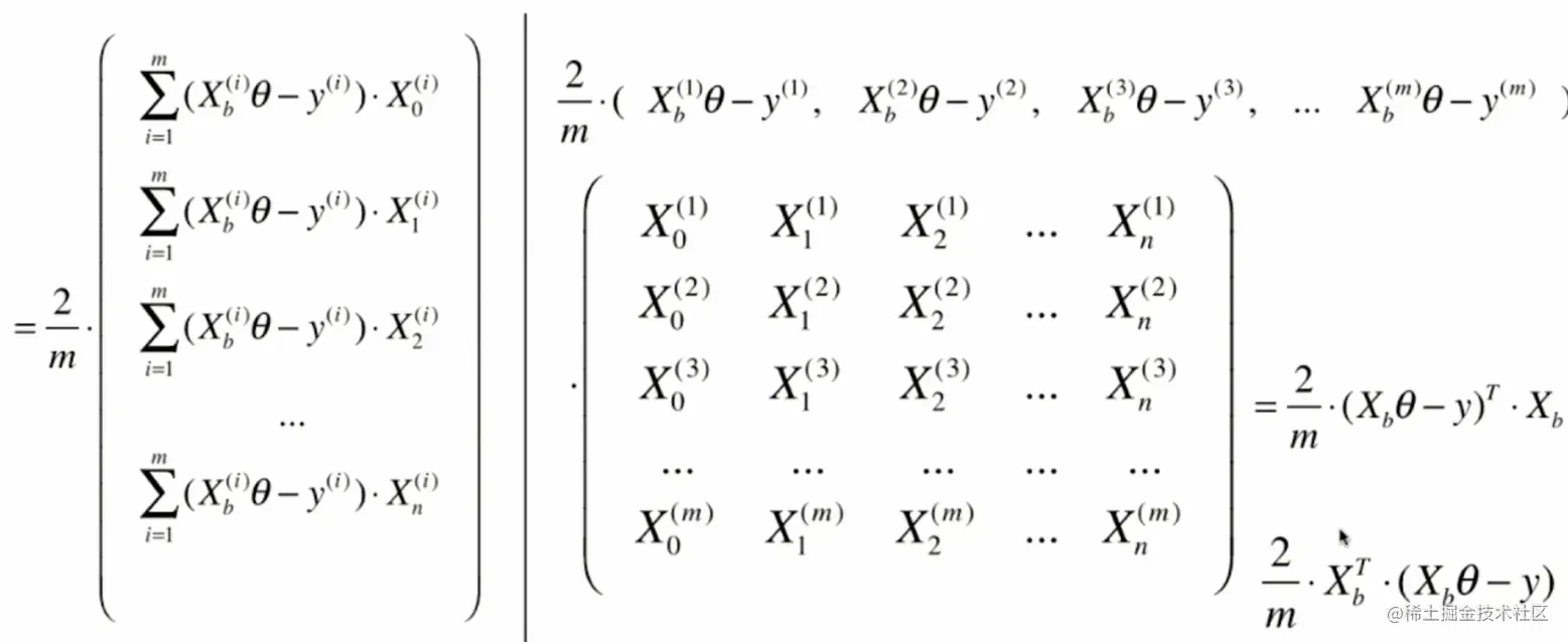
5.梯度下降的向量化和数据标准化
import numpy as np
from sklearn import datasets

boston = datasets.load_boston()
X = boston.data
y = boston.target

X = X[y < 50.0]
y = y[y < 50.0]

from playML.model_selection import train_test_split

X_train, X_test, y_train, y_test = train_test_split(X, y, seed=666)
from playML.LinearRegression import LinearRegression

lin_reg1 = LinearRegression()
%time lin_reg1.fit_normal(X_train, y_train)
lin_reg1.score(X_test, y_test)
使用梯度下降法前进行数据归一化
from sklearn.preprocessing import StandardScaler

standardScaler = StandardScaler()
standardScaler.fit(X_train)
X_train_standard = standardScaler.transform(X_train)

lin_reg3 = LinearRegression()
%time lin_reg3.fit_gd(X_train_standard, y_train)
X_test_standard = standardScaler.transform(X_test)
lin_reg3.score(X_test_standard, y_test)
封装我们自己的SGD
import numpy as np
from .metrics import r2_score

class LinearRegression:

    def __init__(self):
        """初始化Linear Regression模型"""
        self.coef_ = None
        self.intercept_ = None
        self._theta = None

    def fit_normal(self, X_train, y_train):
        """根据训练数据集X_train, y_train训练Linear Regression模型"""
        assert X_train.shape[0] == y_train.shape[0], \
            "the size of X_train must be equal to the size of y_train"

        X_b = np.hstack([np.ones((len(X_train), 1)), X_train])
        self._theta = np.linalg.inv(X_b.T.dot(X_b)).dot(X_b.T).dot(y_train)

        self.intercept_ = self._theta[0]
        self.coef_ = self._theta[1:]

        return self

    def fit_gd(self, X_train, y_train, eta=0.01, n_iters=1e4):
        """根据训练数据集X_train, y_train, 使用梯度下降法训练Linear Regression模型"""
        assert X_train.shape[0] == y_train.shape[0], \
            "the size of X_train must be equal to the size of y_train"

        def J(theta, X_b, y):
            try:
                return np.sum((y - X_b.dot(theta)) ** 2) / len(y)
            except:
                return float('inf')

        def dJ(theta, X_b, y):
            return X_b.T.dot(X_b.dot(theta) - y) * 2. / len(y)

        def gradient_descent(X_b, y, initial_theta, eta, n_iters=1e4, epsilon=1e-8):

            theta = initial_theta
            cur_iter = 0

            while cur_iter < n_iters:
                gradient = dJ(theta, X_b, y)
                last_theta = theta
                theta = theta - eta * gradient
                if (abs(J(theta, X_b, y) - J(last_theta, X_b, y)) < epsilon):
                    break

                cur_iter += 1

            return theta

        X_b = np.hstack([np.ones((len(X_train), 1)), X_train])
        initial_theta = np.zeros(X_b.shape[1])
        self._theta = gradient_descent(X_b, y_train, initial_theta, eta, n_iters)

        self.intercept_ = self._theta[0]
        self.coef_ = self._theta[1:]

        return self

    def predict(self, X_predict):
        """给定待预测数据集X_predict,返回表示X_predict的结果向量"""
        assert self.intercept_ is not None and self.coef_ is not None, \
            "must fit before predict!"
        assert X_predict.shape[1] == len(self.coef_), \
            "the feature number of X_predict must be equal to X_train"

        X_b = np.hstack([np.ones((len(X_predict), 1)), X_predict])
        return X_b.dot(self._theta)

    def score(self, X_test, y_test):
        """根据测试数据集 X_test 和 y_test 确定当前模型的准确度"""

        y_predict = self.predict(X_test)
        return r2_score(y_test, y_predict)

    def __repr__(self):
        return "LinearRegression()"
    ```
文章出处登录后可见!